Calculate local G statistic

This local spatial statistic measures the concentration of high or low values for a given region. This can for example be used to define spatial structures in a tissue section based on the values of selected features. Furthermore, the local G statistic can be used for high/low clustering of data.

NB: This function only calculates G, not G star.

Usage

RunLocalG(object, ...)

# Default S3 method
RunLocalG(
  object,
  spatnet,
  alternative = c("two.sided", "greater", "less"),
  return_as_tibble = TRUE,
  verbose = TRUE
)

# S3 method for class 'Seurat'
RunLocalG(
  object,
  features,
  alternative = NULL,
  store_in_metadata = TRUE,
  assay_name = "GiScores",
  verbose = TRUE,
  ...
)

Arguments

object: An object
...: Parameters passed to GetSpatialNetwork
spatnet: A list of tibbles containing spatial networks generated with GetSpatialNetwork
alternative: A string specifying the alternative hypothesis: "two.sided", "greater" or "less". By default, only the local G scores are returned. If an alternative test is specified, the function will return both local G scores and p-values. Note that p-values are adjusted for multiple hypothesis testing within each feature using "BH" correction. If you want to adjust p-values with a different strategy, you can compute the p-values directly from the local G z-scores.
return_as_tibble: Logical specifying whether the results should be returned as an object of class tbl
verbose: Print messages
features: A character vector of feature names fetchable with FetchData
store_in_metadata: A logical specifying if the results should be returned in the meta data slot. If set to FALSE, the results will instead be returned as an assay named by assay_name. If a statistical test is applied, the adjusted p-values will be returned to the meta data slot if store_in_metadata = TRUE and in the @misc slot of the assay if store_in_metadata = FALSE.
assay_name: Name of the assay if store_in_metadata=FALSE

Value

An object with local G statistics

default method

Takes a matrix-like object with one feature per column and a list of spatial networks generated with GetSpatialNetwork and computes the local G scores and optionally p-values. The G scores are prefixed with "Gi" and p-values are prefixed with one of "Pr(z <!=", "Pr(z " or "Pr(z <" depending on the chosen test.

Seurat

Takes a Seurat object as input and returns the local G scores for a selected number of features and optionally p-values. The G scores are prefixed with "Gi" and p-values are prefixed with one of "Pr(z <!=", "Pr(z " or "Pr(z <" depending on the chosen test.

References

Ord, J. K. and Getis, A. 1995 Local spatial autocorrelation statistics: distributional issues and an application. Geographical Analysis, 27, 286–306
Bivand RS, Wong DWS 2018 Comparing implementations of global and local indicators of spatial association. TEST, 27(3), 716–748 doi:10.1007/s11749-018-0599-x

Author

Ludvig Larsson

Examples

# \donttest{
library(semla)
library(tibble)
library(dplyr)
library(ggplot2)
library(viridis)
#> Loading required package: viridisLite

# read coordinates
coordfile <- system.file("extdata/mousebrain/spatial",
                         "tissue_positions_list.csv",
                         package = "semla")
coords <- read.csv(coordfile, header = FALSE) |>
  filter(V2 == 1) |>
  select(V1, V6, V5) |>
  setNames(nm = c("barcode", "x", "y")) |>
  bind_cols(sampleID = 1) |>
  as_tibble()

# get spatial network
spatnet <- GetSpatialNetwork(coords)

# Load expression data
feature_matrix <- system.file("extdata/mousebrain",
                              "filtered_feature_bc_matrix.h5",
                              package = "semla") |>
  Seurat::Read10X_h5()
featureMat <- t(as.matrix(feature_matrix[c("Mgp", "Th", "Nrgn"), ]))
featureMat <- featureMat[coords$barcode, ]
head(featureMat)
#>                    Mgp Th Nrgn
#> CATACAAAGCCGAACC-1   0  0   19
#> CTGAGCAAGTAACAAG-1   0  0  309
#> GGGTACCCACGGTCCT-1   0  0  108
#> ACGGAATTTAGCAAAT-1   0  0  246
#> GGGCGGTCCTATTGTC-1   0  0  190
#> ATGTTACGAGCAATAC-1   0  0  130

# Calculate G scores
g_scores <- RunLocalG(log1p(featureMat), spatnet)
#> ℹ Setting alternative hypothesis to 'two.sided'
#> →   Calculating local G scores for 2559 spots in sample 1
#> ℹ Calculating p-values for local G scores, MH-adjusted within each feature
#> ℹ G scores will be named Gi[Ftr] and adjusted p-values will be named Pr(z != E(Gi[Ftr]))
head(g_scores)
#> # A tibble: 6 × 7
#>   barcode          `Gi[Mgp]` `Pr(z != E(Gi[Mgp]))` `Gi[Th]` `Pr(z != E(Gi[Th]))`
#>   <chr>                <dbl>                 <dbl>    <dbl>                <dbl>
#> 1 CATACAAAGCCGAAC…    -0.893                 0.757   -0.377                0.894
#> 2 CTGAGCAAGTAACAA…    -0.711                 0.757   -0.533                0.812
#> 3 GGGTACCCACGGTCC…    -1.09                  0.608   -0.462                0.856
#> 4 ACGGAATTTAGCAAA…    -0.645                 0.757   -0.654                0.759
#> 5 GGGCGGTCCTATTGT…    -1.26                  0.608   -0.533                0.812
#> 6 ATGTTACGAGCAATA…    -1.10                  0.608   -0.654                0.759
#> # ℹ 2 more variables: `Gi[Nrgn]` <dbl>, `Pr(z != E(Gi[Nrgn]))` <dbl>

# Bind results with coords for plotting
gg <- coords |>
  bind_cols(log1p(featureMat)) |>
  left_join(y = g_scores, by = "barcode")

# Plot some results
p1 <- ggplot(gg, aes(x, y, color = Th)) + ggtitle("Expression")
p2 <- ggplot(gg, aes(x, y, color = `Gi[Th]`)) + ggtitle("Local G")
p3 <- ggplot(gg, aes(x, y, color = -log10(`Pr(z != E(Gi[Th]))`))) + ggtitle("-log10(p-value)")

p <- p1 + p2 + p3 &
  geom_point() &
  theme_void() &
  scale_y_reverse() &
  coord_fixed() &
  scale_colour_gradientn(colours = viridis(n = 9))
p

# }


library(semla)
library(dplyr)

# Load Seurat object with mouse bain data
se_mbrain <- readRDS(system.file("extdata/mousebrain", "se_mbrain", package = "semla"))
se_mbrain <- se_mbrain |>
  ScaleData(verbose = FALSE) |>
  FindVariableFeatures(verbose = FALSE) |>
  RunPCA(verbose = FALSE)

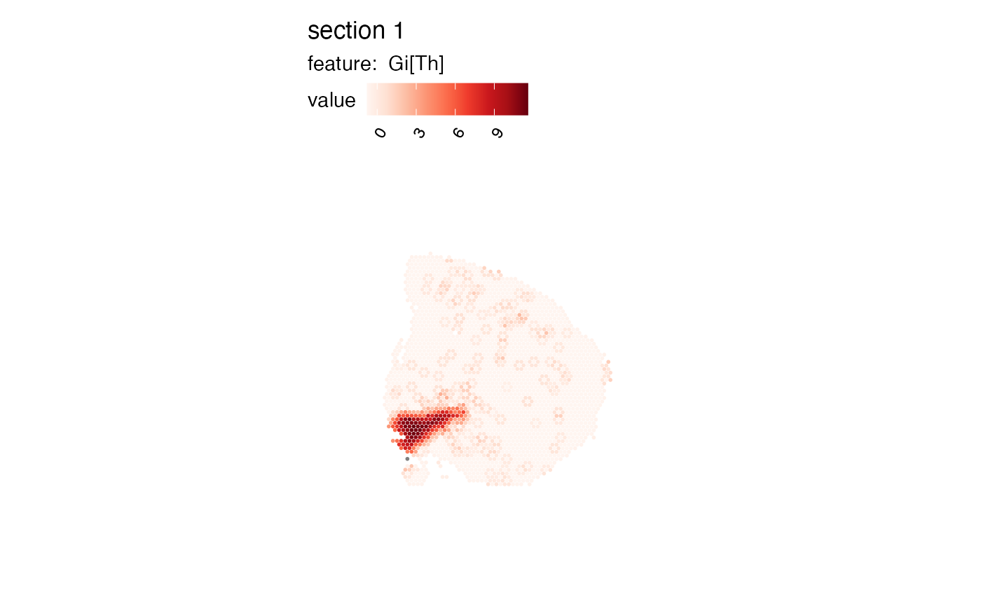
# Calculate G scores
se_mbrain <- RunLocalG(se_mbrain, features = c("Th", "Mgp"), alternative = "greater")
#> 
#> ── Calculating local G ──
#> 
#> ℹ Got 2 feature(s)
#> ℹ Setting alternative hypothesis to 'greater'
#> →   Calculating local G scores for 2559 spots in sample 1
#> ℹ Calculating p-values for local G scores, MH-adjusted within each feature
#> ℹ G scores will be named Gi[Ftr] and adjusted p-values will be named Pr(z > E(Gi[Ftr]))
#> ℹ Placing results in 'Seurat' object meta.data slot
#> ✔ Returning results

# Plot G scores
MapFeatures(se_mbrain, features = "Gi[Th]")


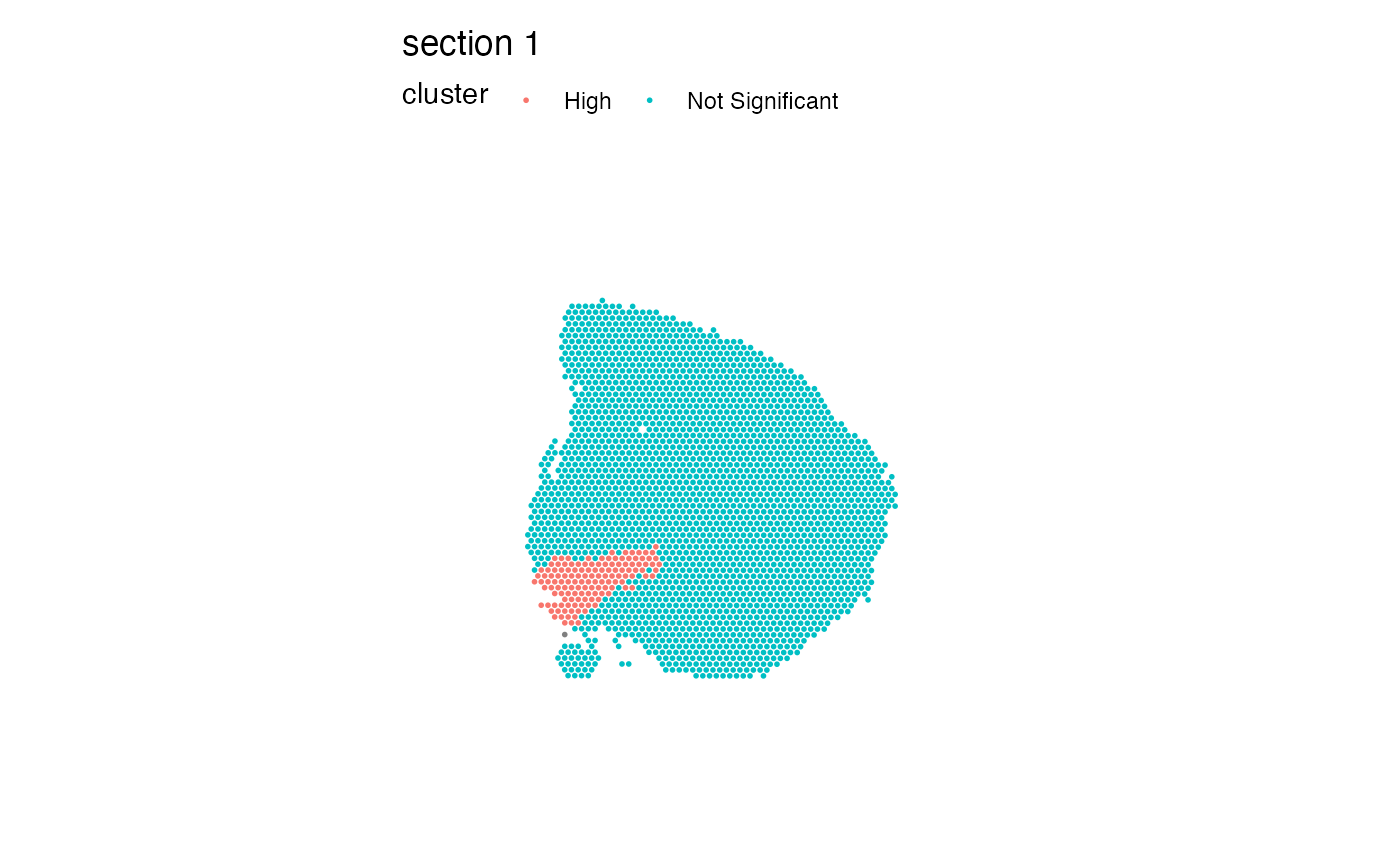
# high/low clustering
se_mbrain$cluster <- se_mbrain[[]] |>
  mutate(cluster = case_when(
    `Pr(z > E(Gi[Th]))` > 0.05 ~ "Not Significant",
    `Pr(z > E(Gi[Th]))` <= 0.05 & `Gi[Th]` > 0 ~ "High"
  )) |> pull(cluster)
MapLabels(se_mbrain, column_name = "cluster")