Non-negative matrix factorization

Non-negative matrix factorization (NNMF or NMF) can be a useful technique to deconvolve 10x Visium data, in particular when a reference single-cell RNA-seq data is not available to conduct cell type deconvolution. In this vignette we will demonstrate how you can apply this method with semla on spatial data.

We recommend using the singlet R package for NNMF which handles Seurat objects. singlet uses the ultra fast NNMF implementation from RcppML. Both of these packages are developed by Zach DeBruines lab and you can find more information about their work and tools at https://github.com/zdebruine and https://www.zachdebruine.com/.

RcppML is available on CRAN and GitHub, and singlet can be installed from GitHub with devtools::install_github("zdebruine/singlet").

library(semla)
library(singlet)
library(SeuratData)

Run NMF

We’ll use a mouse brain Visium data set provided in SeuratData for the NNMF. The method automatically runs cross-validation to find the best rank and learns a model at that rank.

The factorization can be computed on all genes, but below we have filtered the data to include only the top variable features to speed up the computation.

# Here we'll use an example data set provided in SeuratData
se_mbrain <- LoadData("stxBrain", type = "anterior1")

# Update se_mbrain for compatibility with semla
se_mbrain <- UpdateSeuratForSemla(se_mbrain)

# Normalize data and find top variable features
se_mbrain <- se_mbrain |> 
  NormalizeData() |> 
  FindVariableFeatures()

# OPTIONAL: subset data to improve computational speed
se_mbrain <- se_mbrain[VariableFeatures(se_mbrain), ]

# Set seed for reproducibility
set.seed(42)
se_mbrain <- RunNMF(se_mbrain)

k <- ncol(se_mbrain@reductions$nmf@feature.loadings)

We can plot the cross-validation results and find that the optimal rank decided by the method is 22, which determines the number of factors we obtain from the NMF run.

RankPlot(se_mbrain)

Spatial visualization

The results are stored as a DimReduc object in our Seurat object and we can map the factors spatially with MapFeatures().

MapFeatures(se_mbrain, 
            features = paste0("NMF_", 1:22), 
            override_plot_dims = TRUE, 
            colors = viridis::magma(n = 11, direction = -1)) &
  theme(plot.title = element_blank())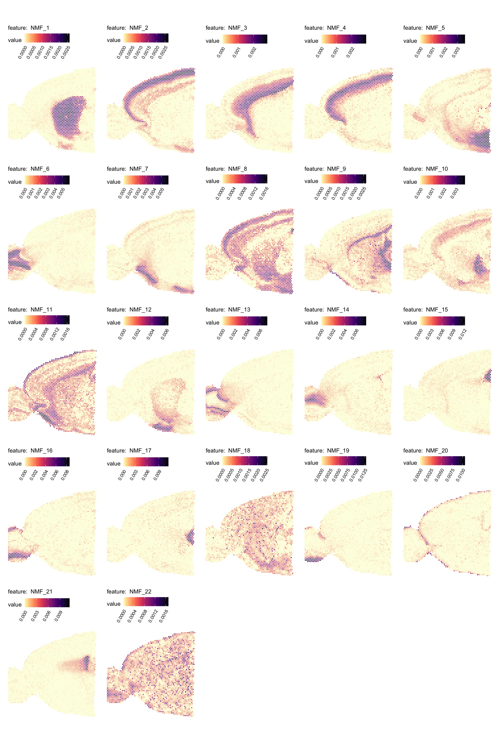

Explore gene contributions

We can also investigate the gene loadings for each factor with PlotFeatureLoadings() which will give us an idea about what the top contributing genes for each factor are. Below we can see the top 30 contributing genes for NMF_1 and NMF_2.

PlotFeatureLoadings(se_mbrain, 
                    dims = 1:2, 
                    reduction = "nmf", 
                    nfeatures = 30,
                    mode = "dotplot", 
                    fill = "darkmagenta",
                    pt_size = 3)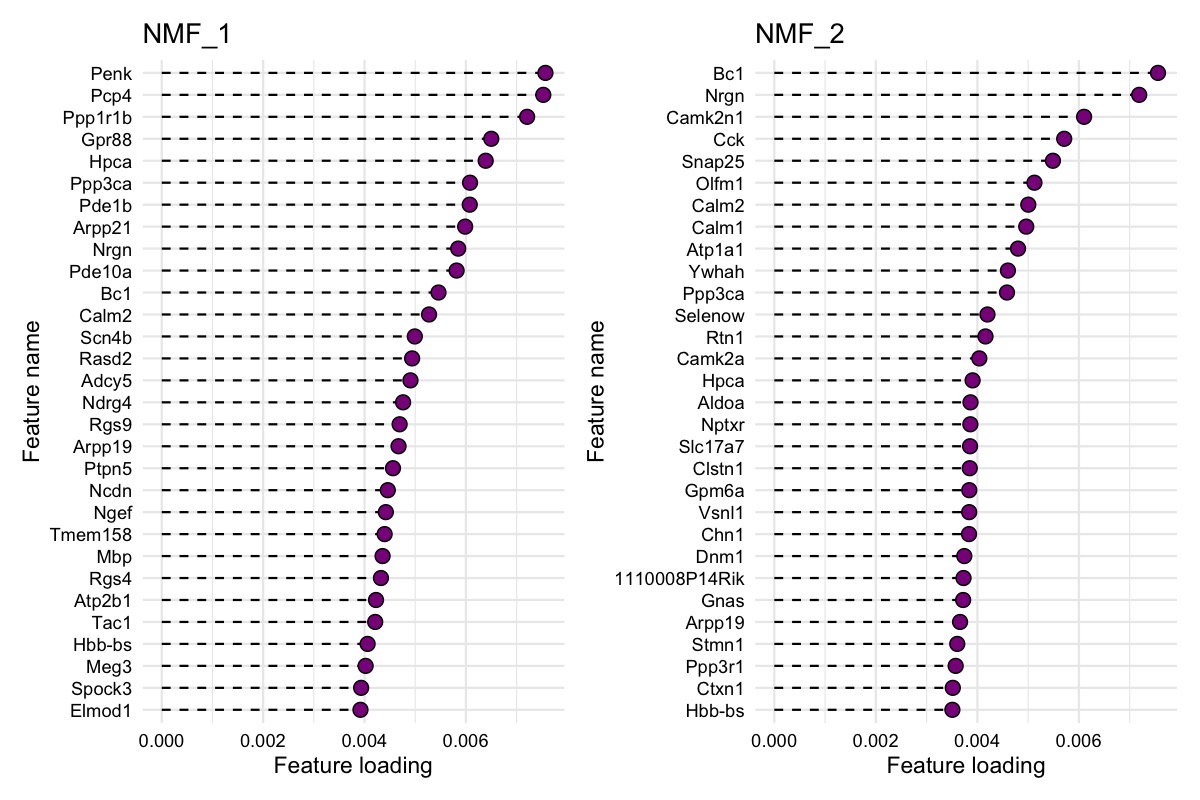

Make composite plot

We can also map multiple factors spatially in a single plot with MapMultipleFeatures(). Note that the visualization will only display the most dominant factor for each spot. See ?MapMultipleFeatures() for details.

se_mbrain <- LoadImages(se_mbrain)

factor_colors <- c('#e6194b', '#3cb44b', '#ffe119', '#4363d8', '#f58231', 
                   '#911eb4', '#46f0f0', '#f032e6', '#bcf60c', '#fabebe', 
                   '#008080', '#e6beff', '#9a6324', '#fffac8', '#800000', '#aaffc3')

# Select non-overlapping factors
selected_factors <- c(1, 2, 3, 4, 5, 6, 7, 9, 10, 12, 13, 15, 16, 17, 19, 20)

MapMultipleFeatures(se_mbrain, 
                    features = paste0("NMF_", selected_factors), 
                    colors = factor_colors, 
                    image_use = "raw", 
                    override_plot_dims = TRUE, 
                    pt_size = 2)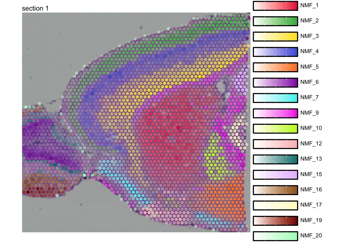

Explore gene contributions (heatmap)

Similarly, we can also summarize the top feature loadings for each factor with a heatmap:

PlotFeatureLoadings(se_mbrain, 
                    dims = selected_factors, 
                    reduction = "nmf", 
                    nfeatures = 30, 
                    mode = "heatmap", 
                    gradient_colors = viridis::magma(n = 11, direction = -1))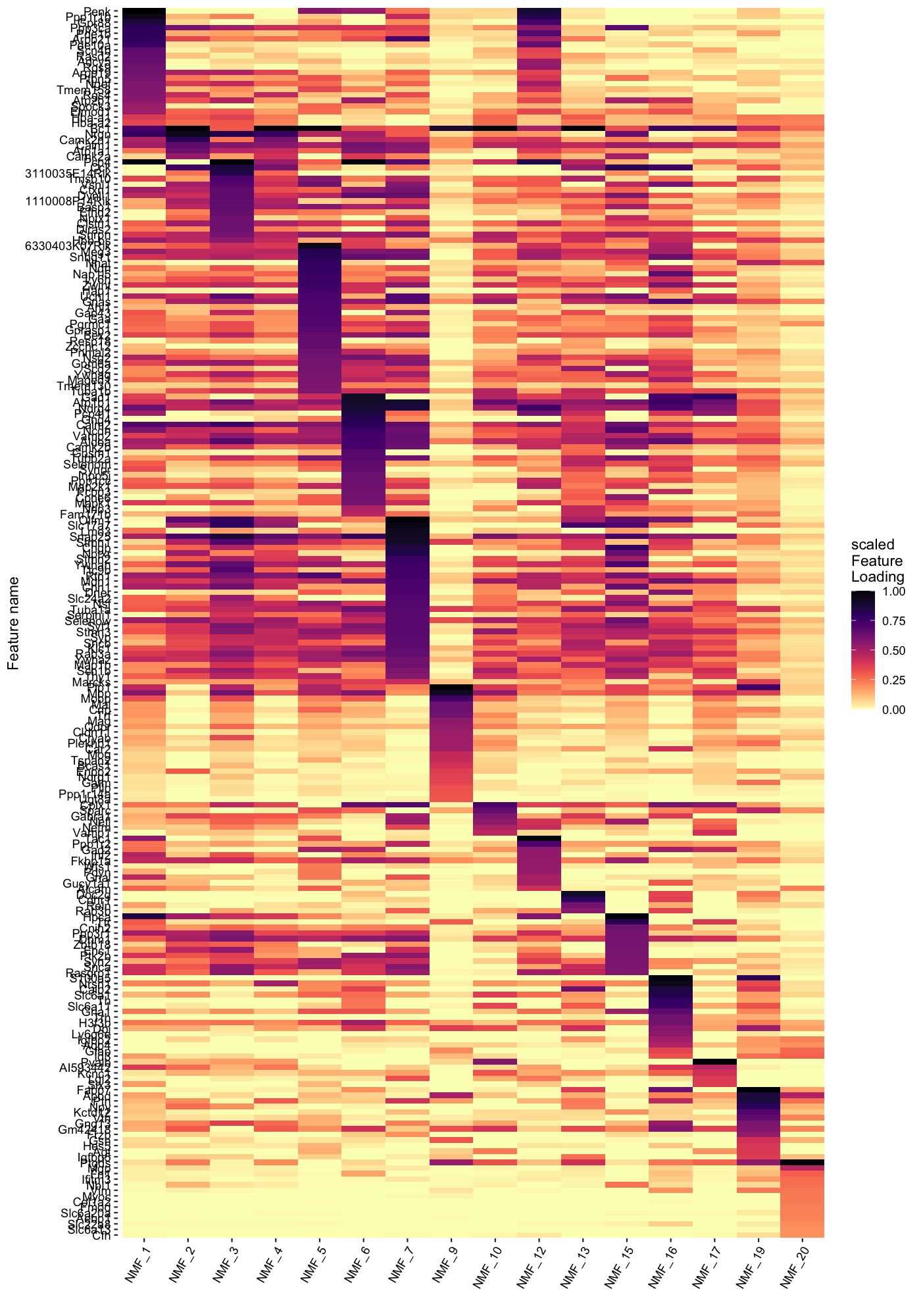

Functional Enrichment Analysis (FEA)

If you want to get the feature loading values for each factor, you can extract them from the DimReduc object. This can for example be useful to run Functional Enrichment Analysis (FEA).

# fetch feature.loadings from DimReduc object
nmf_loadings <- se_mbrain[["nmf"]]@feature.loadings

# Convert to long format and group data by factor
gene_loadings_sorted <- nmf_loadings |> 
  as.data.frame() |> 
  tibble::rownames_to_column(var = "gene") |> 
  as_tibble() |> 
  tidyr::pivot_longer(all_of(colnames(nmf_loadings)), names_to = "fctr", values_to = "loading") |> 
  mutate(fctr = factor(fctr, colnames(nmf_loadings))) |> 
  group_by(fctr) |> 
  arrange(fctr, -loading)

# Extract top 10 genes per factor
gene_loadings_sorted |> 
  slice_head(n = 10)

## # A tibble: 220 × 3
## # Groups:   fctr [22]
##    gene    fctr  loading
##    <chr>   <fct>   <dbl>
##  1 Penk    NMF_1 0.00757
##  2 Pcp4    NMF_1 0.00753
##  3 Ppp1r1b NMF_1 0.00721
##  4 Gpr88   NMF_1 0.00650
##  5 Hpca    NMF_1 0.00639
##  6 Ppp3ca  NMF_1 0.00608
##  7 Pde1b   NMF_1 0.00608
##  8 Arpp21  NMF_1 0.00598
##  9 Nrgn    NMF_1 0.00585
## 10 Pde10a  NMF_1 0.00582
## # ℹ 210 more rows

Run functional enrichment analysis on top 10 genes from factor 1:

library(gprofiler2)

# Get gene sets
gene_set_nmf_1 <- gene_loadings_sorted |> 
  filter(fctr == "NMF_1") |> 
  slice_head(n = 10)

# Run FEA
fea_results_nmf_1 <- gost(query = gene_set_nmf_1$gene, ordered_query = TRUE, organism = "mmusculus", sources = "GO:BP")$result |> 
  as_tibble()

# Look at results
fea_results_nmf_1 |> select(p_value, term_size, query_size, intersection_size, term_name)

## # A tibble: 23 × 5
##      p_value term_size query_size intersection_size term_name                   
##        <dbl>     <int>      <int>             <int> <chr>                       
##  1 0.0000825        36          7                 3 response to amphetamine     
##  2 0.000265        250          7                 4 locomotory behavior         
##  3 0.000301        188          9                 4 learning                    
##  4 0.000302         55          7                 3 response to amine           
##  5 0.000384       1329          8                 6 response to abiotic stimulus
##  6 0.000885        417          6                 4 response to salt            
##  7 0.00214         760          9                 5 behavior                    
##  8 0.00264         324          9                 4 learning or memory          
##  9 0.00342         475          7                 4 response to radiation       
## 10 0.00401         360          9                 4 cognition                   
## # ℹ 13 more rows

Package versions

semla: 1.1.6
RcppML: 0.5.6
singlet: 0.99.27

Session info

sessionInfo()