Cell type mapping benchmark

Last compiled: 18 September 2024

Load required packages

library(semla)
if (!requireNamespace('TabulaMurisSenisData', quietly = TRUE)) {
  BiocManager::install("TabulaMurisSenisData")
}
library(TabulaMurisSenisData)
library(SingleCellExperiment)
library(patchwork)
library(spacexr)
library(pbapply)

Load single-cell data (Allen Brain atlas) and Visium data (mouse brain tissue section).

Load data

We have access to 23 annotated cell types in the single-cell data.

DimPlot(se_allen, group.by = "subclass")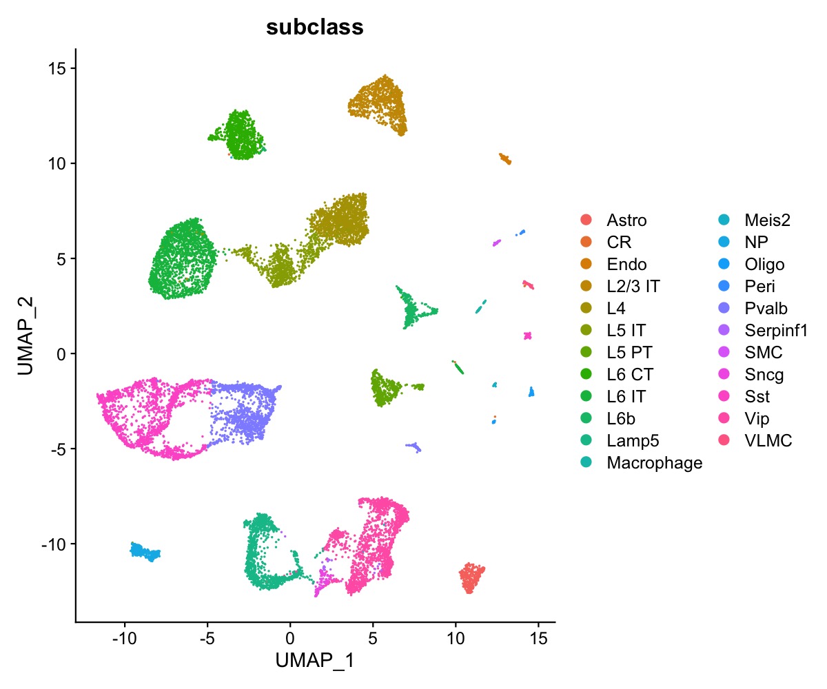

1. The reference single-cell data set contains 23 annotated cell types.

Create dummy expression profiles

Here we’ll create a synthetic Visium data set by sample single-cells from the Allen Brain atlas data set:

1. Downsample UMIs to 1%. This is to make sure that the synthetic data have roughly the same library sizes as the Visium mouse brain tissue section data set.
2. Calculate cell type weights. These weights will be used to determine the probability of a cell type being samples for the synthetic spots. Abundant cell type will be assigned higher probabilities and vice versa.
3. Sample cell numbers per synthetic spot. Here we’ll draw counts from a poisson distribution with the lambda (mean) parameter set to 10.
4. Select cell indices. The indices will be randomly selected using the cell type weights defined in step 2.
5. Aggregate expression vectors for selected indices. Each synthetic spot will consist of the averaged gene expression vectors obtained from the sampled cells.
6. Combine aggregated expression profiles to a final synthetic count matrix.

se_allen <- FindVariableFeatures(se_allen, nfeatures = 5e3)
se_allen <- se_allen[VariableFeatures(se_allen), ]
umis <- GetAssayData(se_allen, slot = "counts")

# 1. Down sample UMIs
bins <- split(1:ncol(se_allen), cut(1:ncol(se_allen), breaks = 50))
batches <- pblapply(bins, function(inds) {
  umis_subset <- scuttle::downsampleMatrix(umis[, inds], prop = 0.01)
  return(umis_subset)
}, cl = 7)
downsampled_umis <- do.call(cbind, batches)

# 2. Calculate cell type weights
props <- table(se_allen$subclass)
props <- props/sum(props) |> as.numeric()

# 3. Sample cells
# Set the average count
average_count <- 10

# Set the number of samples
num_samples <- 1e4

# Generate samples from a Poisson distribution with the specified average
set.seed(123)
sampled_counts <- rpois(num_samples, lambda = average_count)
sampled_counts[sampled_counts == 0] <- 1

# 4. Select cell indices
label_matrix <- sapply(names(props), function(label) se_allen$subclass == label)
sampled_indices <- pblapply(1:length(sampled_counts), function(i) {
  x <- sample(x = names(props), size = sampled_counts[i], prob = props, replace = TRUE)
  y <- table(x)
  inds <- c()
  for (lbl in unique(x)) {
    inds <- c(inds, sample(x = which(label_matrix[, lbl]), size = y[lbl]))
  }
  return(inds)
}, cl = 7)

# 5. Aggregate expression vectors
bins <- split(1:num_samples, cut(1:num_samples, breaks = 50))
batches <- pblapply(bins, function(inds) {
  umis_subset <- downsampled_umis[, sampled_indices[inds] |> unlist()]
  umis_subset <- rowsum(umis_subset |> t(), group = rep(x = inds, sampled_indices[inds] |> sapply(length))) |> t()
  return(umis_subset)
}, cl = 7)

# 6. Combine aggregated expression profiles
mini_bulk_umis <- do.call(cbind, batches)

Export Allen brain atlas data for cell2location and stereoscope

Here we’ll export a subset of the single-cell data including 250 randomly selected cells per cell type. If a cell type has less than 250 cells, all cells will be selected. Only cell types with more than 10 cells are kept.

The exported matrices and tables will be used to run stereoscope and cell2location in a separate environment.

seed = 1337L
nCells_per_group <- 250
set.seed(seed)

# Sample barcodes
barcodes <- tibble(barcode = colnames(se_allen), group = se_allen$subclass) |>
  group_by(group) |>
  slice(sample(min(nCells_per_group, n())))

# Remove low abundant cell types
cells_per_celltype <- table(barcodes$group)
keep <- names(cells_per_celltype)[cells_per_celltype > 10]
barcodes <- barcodes |> filter(group %in% keep)

# Export matrices and tables
dir.create("synthetic_spots")
data.table::fwrite(GetAssayData(se_allen, slot = "counts")[, barcodes$barcode] |> t() |> as.data.frame(), file = "synthetic_spots/allen_brain_umis.tsv", quote = FALSE, sep = "\t", row.names = TRUE, col.names = TRUE)
writeLines(rownames(se_allen), con = "synthetic_spots/variable_genes.txt")
data.table::fwrite(se_allen@meta.data[barcodes$barcode, ] |> select(subclass), file = "synthetic_spots/metadata.tsv", sep = "\t", quote = FALSE, row.names = TRUE, col.names = TRUE)
data.table::fwrite(GetAssayData(se_Visium_agg, slot = "counts") |> t() |> as.data.frame(), file = "synthetic_spots/Visium_synthetic_spots_umis.tsv", quote = FALSE, sep = "\t", row.names = TRUE, col.names = TRUE)

Create a Seurat object from the synthetic count matrix

Each synthetic spot will be named “barcode1”, barcode2”, …

For downstream steps, we need to normalize the data and select a set of top 5,000 variable genes.

colnames(mini_bulk_umis) <- paste0("barcode", 1:num_samples)
se_Visium_agg <- CreateSeuratObject(counts = mini_bulk_umis, assay = "Spatial")

se_Visium_agg <- se_Visium_agg |>
  NormalizeData() |>
  FindVariableFeatures(nfeatures = 5000)

Run NNLS

The RunNNLS() method requires a Seurat object with normalized 10x Visium data and a Seurat object with normalized single-cell data. The groups argument defines what meta data column the cell type labels should be taken from in the single-cell Seurat object. In our single-cell Seurat object, the labels are stored in the “subclass” column.

Computation time

For the NNLS method, we’ll run 10 rounds, adding 10,000 spots to each round and starting with 10,000 spots. Below we create a “large” Seurat object with 100,000 spots by merging our se_Visium_agg object 10 times.

# Merge Seurat object to have 100k spots
se_Visium_agg_large <- merge(se_Visium_agg, y = list(se_Visium_agg, se_Visium_agg, se_Visium_agg, se_Visium_agg, se_Visium_agg, se_Visium_agg, se_Visium_agg, se_Visium_agg, se_Visium_agg))
DefaultAssay(se_Visium_agg_large) <- "Spatial"
se_Visium_agg_large <- FindVariableFeatures(se_Visium_agg_large, nfeatures = 5e3)

Since the NNLS method runs in a matter of seconds, we’ll run each round in 10 iterations to compute average computation times.

nnls_results <- list()
for (i in seq(1e4, 1e5, 1e4)) {
  print(i)
  DefaultAssay(se_Visium_agg_large) <- "Spatial"
  se_Visium_agg_subset <- se_Visium_agg_large[, 1:i]
  iters <- sapply(1:10, function(n) {
    cat(paste0("  iter: ", n, "\n"))
    ti <- Sys.time()
    tmp <- RunNNLS(object = se_Visium_agg_subset, nCells_per_group = 250, 
                   singlecell_object = se_allen, 
                   groups = "subclass", verbose = FALSE)
    stamp <- Sys.time() - ti
    return(stamp)
  })
  nnls_results[[paste0("n", i)]] <- tibble(n = i, stamp = iters)
  rm(se_Visium_agg_subset)
}
nnls_stamps <- do.call(bind_rows, nnls_results)

Now we can plot the average computation times for each data set size.

p <- ggplot(nnls_stamps |> group_by(n) |> summarize(mean = mean(stamp), sd = sd(stamp)), 
       aes(x = n, y = mean, ymin = mean - sd, ymax = mean + sd)) + 
  geom_errorbar(width = 0) +
  geom_point() +
  labs(x = "Number of spots", y = "Seconds", title = "Computation time with NNLS (5,000 genes)") +
  theme_minimal() +
  scale_x_continuous(labels=function(x) format(x, big.mark = ",", scientific = FALSE), 
                     breaks = seq(1e4, 1e5, 1e4)) +
  theme(axis.text.x = element_text(angle = 50, hjust = 1), panel.border = element_rect(fill = NA, colour = "black"))
p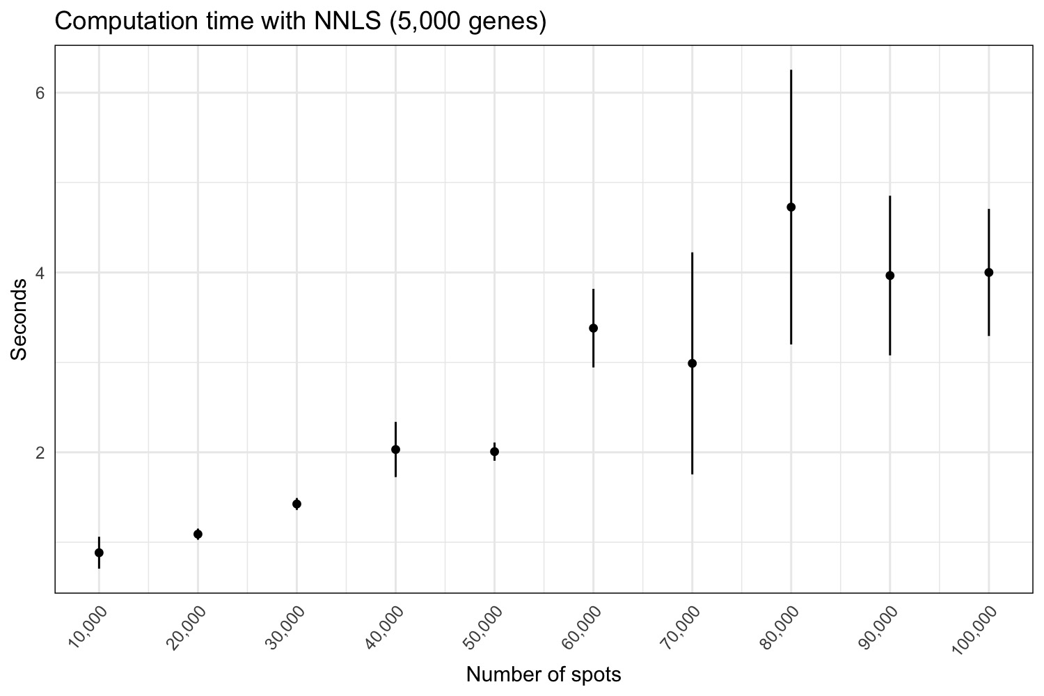

2. Computation time for NNLS on synthetic Visium data. The x-axis shows the number of spots and the y-axis shows the run time in seconds.

Compute performance metrics

For the performance assessment, we’ll run the NNLS method on our 10,000 spots se_Visium_agg data set. We can get the expected counts by counting the number of cell types using our sampled indices.

# Calculate expected counts per spot
expected_counts <- do.call(bind_rows, pblapply(seq_along(sampled_indices), function(i) {
  x <- se_allen$subclass[sampled_indices[[i]]] |> table()
  tibble(spot = paste0("barcode", i), celltype = names(x), lbl = x |> as.integer())
}, cl = 7))

# Run NNLS for 1e4 spots
DefaultAssay(se_Visium_agg) <- "Spatial"
se_Visium_agg <-  RunNNLS(object = se_Visium_agg, 
                   singlecell_object = se_allen, 
                   groups = "subclass", verbose = FALSE, min_prop = 0)

# cast to wide format
props <- expected_counts |> tidyr::pivot_wider(id_cols = spot, names_from = celltype, values_from = lbl) |> 
  tibble::column_to_rownames(var = "spot") |> 
  as.matrix()
props[is.na(props)] <- 0
props <- prop.table(props, margin = 1)
props <- props[, colnames(props) != "CR"]
props <- props[, rownames(se_Visium_agg)]

# Compare proportions
pred_all <- tibble(inf_props_nnls = GetAssayData(se_Visium_agg, slot = "data") |> 
                     as.matrix() |> t() |> as.numeric(),
             exp_props = props |> as.numeric(), 
             celltype = rep(rownames(se_Visium_agg), each = 1e4))

Run RCTD

Now we can run the RCTD method on our 10,000 spots data set and time the computation. The RCTD method could not be run locally for larger data sets and we therefore only ran the deconvolution for 10,00 spots. (Took ~19 minutes to run on a Macbook Pro 2017, 3.1 GHz Quad-Core Intel Core i7, 16GB).

# set up reference
Idents(se_allen) <- "subclass"

# extract information to pass to the RCTD Reference function
celltypes <- gsub(pattern = "\\/", replacement = ".", x = se_allen$subclass)
celltypes <- celltypes[celltypes != "CR"]
cluster <- as.factor(gsub(pattern = "\\/", replacement = ".", x = celltypes))
nUMI <- colSums(GetAssayData(se_allen, slot = "counts"))
reference <- Reference(GetAssayData(se_allen, slot = "counts")[, barcodes$barcode], cluster[barcodes$barcode], nUMI[barcodes$barcode])

# set up query with the RCTD function SpatialRNA
colnames(mini_bulk_umis) <- paste0("barcode", 1:ncol(mini_bulk_umis))
coords <- data.frame(x = 1:1e4, y = 1:1e4, row.names = paste0("barcode", 1:1e4))

query <- SpatialRNA(coords = coords, counts = mini_bulk_umis, nUMI = colSums(mini_bulk_umis))

# Run RCTD
ti <- Sys.time()
RCTD <- create.RCTD(query, reference, max_cores = 7)
RCTD <- run.RCTD(RCTD, doublet_mode = 'full')
rctd_stamp <- Sys.time() - ti

Compute performance metrics

The results of RCTD full mode are stored in @results$weights. To obtain proportion estimates, we normalize the weights using normalize_weights so that they sum to one. Each entry represents the estimated proportion of each cell type on each spot.

barcodes <- colnames(RCTD@spatialRNA@counts)
weights <- RCTD@results$weights
norm_weights <- normalize_weights(weights)
colnames(norm_weights) <- gsub(pattern = "\\.", replacement = "/", x = colnames(norm_weights))

# Compare proportions
pred_all$inf_props_rctd <- norm_weights[, colnames(props)] |> as.numeric()

Seurat

Finally, we’ll run the label transfer method available from Seurat. The method returns prediction scores for each cell type and spot which cannot be directly interpreted as proportions. However, if we normalize the prediction scores we can use them as a proxy for cell type proportions to calculate our performance metrics.

Computation time

The Seurat method runs relatively fast and we therefore logged the computation time running on synthetic Visium data from 10,000 to 100,000 spots.

se_Visium_agg_large <- SetIdent(se_Visium_agg_large, value = "Spatial")
se_Visium_agg_large <- se_Visium_agg_large |> ScaleData() |> RunPCA()

seurat_results <- list()
for (i in seq(1e4, 1e5, 1e4)) {
  print(i)
  DefaultAssay(se_Visium_agg_large) <- "Spatial"
  se_Visium_agg_subset <- se_Visium_agg_large[, 1:i]
  ti <- Sys.time()
  anchors <- FindTransferAnchors(reference = se_allen, 
                                 query = se_Visium_agg_subset)
  predictions.assay <- TransferData(anchorset = anchors, 
                                    refdata = se_allen$subclass, 
                                    prediction.assay = TRUE,
                                    weight.reduction = se_Visium_agg_subset[["pca"]], 
                                    dims = 1:30)
  stamp <- Sys.time() - ti
  seurat_results[[paste0("n", i)]] <- tibble(n = i, stamp = stamp)
}
seurat_stamps <- do.call(bind_rows, seurat_results)

Below we compare the run time for the NNLS and Seurat methods.

gg <- bind_rows(nnls_stamps |> mutate(method = "nnls") |> mutate(stamp = as.numeric(stamp)),
                seurat_stamps |> mutate(method = "Seurat") |> mutate(stamp = as.numeric(stamp)*60))
p <- ggplot(gg |> group_by(n, method) |> summarize(mean = mean(stamp), sd = sd(stamp)), 
       aes(x = n, y = mean, ymin = mean - sd, ymax = mean + sd, color = method)) + 
  geom_point() +
  geom_line() +
  labs(x = "Number of spots", y = "Seconds", title = "Computation time with NNLS and Seurat (5,000 genes)") +
  theme_minimal() +
  scale_x_continuous(labels=function(x) format(x, big.mark = ",", scientific = FALSE), 
                     breaks = seq(1e4, 1e5, 1e4)) +
  scale_y_log10() +
  annotation_logticks() +
  theme(axis.text.x = element_text(angle = 50, hjust = 1), panel.border = element_rect(fill = NA, colour = "black"))
p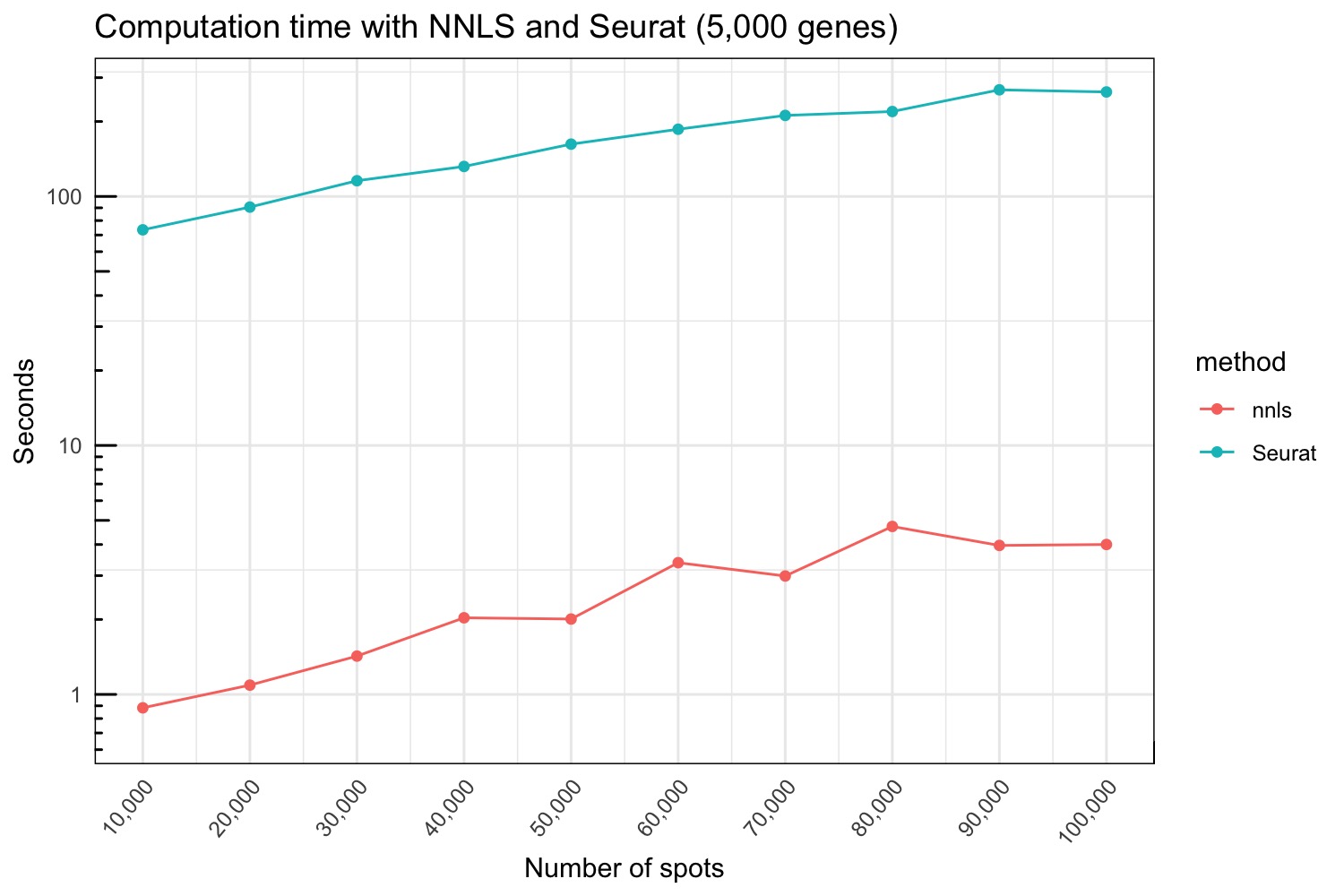

3. Computation time for NNLS and Seurat label transfer on synthetic Visium data. The x-axis shows the number of spots and the y-axis shows the run time in seconds (log10 scale).

Compute performance metrics

Again, we can run the Seurat method on our 10,000 spots data set and normalize the results scores to obtain proportion estimates and calculate performance metrics.

se_Visium_agg <- SetIdent(se_Visium_agg, value = "Spatial")
se_Visium_agg <- se_Visium_agg |> ScaleData() |> RunPCA()
anchors <- FindTransferAnchors(reference = se_allen[, se_allen$subclass != "CR"], 
                               query = se_Visium_agg)
predictions.assay <- TransferData(anchorset = anchors, 
                                  refdata = se_allen$subclass[se_allen$subclass != "CR"], 
                                  prediction.assay = TRUE,
                                  weight.reduction = se_Visium_agg[["pca"]], 
                                  dims = 1:30)
predictions.assay.props <- prop.table(predictions.assay@data[rownames(predictions.assay) != "max", ], margin = 2)

# Compare proportions
pred_all$inf_props_seurat <- predictions.assay.props[rownames(se_Visium_agg@assays$celltypeprops), ] |> t() |> as.numeric()

Stereoscope

For deconvolution with stereoscope, we used the scvi implementation, following the tutorial ‘STereoscope applied to left ventricule data’. First, a model was trained on the scRNA-seq data with 1,000 epochs. Next, the model was used to deconvolve the synthetic Visium expression profiles in 2,000 epochs. For the stereoscope deconvolution, we used a NVIDIA A100-SMX4-80GB Tensor core GPU.

Compute performance metrics

stereoscope <- read.table("synthetic_spots/stereoscope/W.2023-08-17102550.170200.tsv", sep = "\t", header = TRUE, row.names = 1, check.names = FALSE)
pred_all$inf_props_stereoscope <- stereoscope[, rownames(se_Visium_agg@assays$celltypeprops)] |> as.matrix() |> as.numeric()

Cell2location

For deconvolution with cell2location, we followed the tutorial ‘Mapping human lymph node cell types to 10X Visium with Cell2location’. First, a model was trained on the scRNA-seq data with 1,000 epochs. Next, the model was used to deconvolve the synthetic Visium expression profiles in 30,000 epochs. For the cell2location deconvolution, we used a NVIDIA A100-SMX4-80GB Tensor core GPU.

Compute performance metrics

Load cell2location cell abundances.

cell2location <- read.table("synthetic_spots/cell2location/q05_cell_abundance_w_sf.csv", sep = ",", header = TRUE, row.names = 1, check.names = FALSE)
cell2location_props <- prop.table(cell2location |> as.matrix(), margin = 1)
colnames(cell2location_props) <- gsub(pattern = "q05cell_abundance_w_sf_", replacement = "", x = colnames(cell2location_props))
pred_all$inf_props_cell2location <- cell2location_props[, rownames(se_Visium_agg@assays$celltypeprops)] |> as.matrix() |> as.numeric()

Run time for 10k spots

p <- ggplot(run_time, aes(method, time)) +
  geom_col() +
  scale_y_log10() +
  geom_label(aes(method, time, label = time_format)) +
  labs(x = "Deconvolution method", y = "time in seconds", title = "Run time for 10,000 spots")
p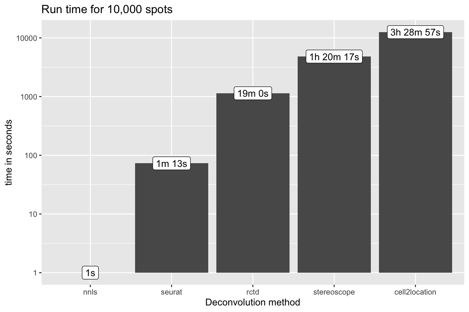

4. Computation time for 5 methods on synthetic Visium data with 10,000 spots. The y-axis shows the run time in seconds.

rmse <- function(x, y) {
  sqrt(mean((x - y)^2))
}

pred_all_long <- pred_all |> 
  tidyr::pivot_longer(cols = c("inf_props_nnls", "inf_props_rctd", "inf_props_seurat", 
                               "inf_props_stereoscope", "inf_props_cell2location"), 
                      names_to = "method", values_to = "inf_props") |> 
  mutate(method = gsub(pattern = "inf_props_", replacement = "", x = method)) |> 
  mutate(method = factor(method, levels = c("nnls", "rctd", "stereoscope", "cell2location", "seurat"))) |> 
  group_by(celltype, method) |> 
  summarize(cor = cor(exp_props, inf_props),
            rmse = rmse(exp_props, inf_props), .groups = "drop")

p1 <- ggplot(pred_all_long, aes(method, cor)) +
  geom_violin(width = 1) +
  labs(title = "Pearson correlation (inferred vs expected proportions)")
p2 <- ggplot(pred_all_long, aes(method, rmse)) +
  geom_violin(width = 1) +
  labs(title = "RMSE (inferred vs expected proportions)")
p1 + p2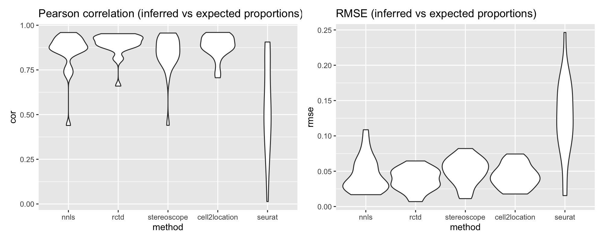

5. Performance metrics for 5 methods. The pearson correlation scores and RMSE are calculated from the inferred vs expected proportions.

Scatter plots

pred_all_long <- pred_all |> tidyr::pivot_longer(cols = c("inf_props_nnls", "inf_props_rctd", "inf_props_seurat", 
                                                "inf_props_stereoscope", "inf_props_cell2location"), 
                                       names_to = "method", values_to = "inf_props") |> 
         mutate(method = gsub(pattern = "inf_props_", replacement = "", x = method))
p <- ggplot(pred_all_long, 
       aes(exp_props, inf_props)) +
  geom_point(size = 0.5) +
  facet_grid(celltype~method) +
  geom_smooth(method = lm) +
  scale_x_continuous(limits = c(0, 1)) +
  scale_y_continuous(limits = c(0, 1)) +
  geom_abline(slope = 1, intercept = 0, linetype = "dashed", color = "red") +
  labs(x = "Expected proportions", y = "Inferred proportions") +
  theme(axis.text.x = element_text(angle = 90, vjust = 0.5))
p

6. Scatter plot showing expected vs inferred cell type proportions for 5 methods on 10,000 synthetic Visium spots. The blue line indicates a fitter trend line and the dashed red lines indicate the expected 1 to 1 relationship.

---

Package versions

• semla: 1.1.6

• RcppML: 0.5.6

Session info

sessionInfo()

## R version 4.4.0 (2024-04-24)
## Platform: aarch64-apple-darwin20
## Running under: macOS Sonoma 14.5
## 
## Matrix products: default
## BLAS:   /Library/Frameworks/R.framework/Versions/4.4-arm64/Resources/lib/libRblas.0.dylib 
## LAPACK: /Library/Frameworks/R.framework/Versions/4.4-arm64/Resources/lib/libRlapack.dylib;  LAPACK version 3.12.0
## 
## locale:
## [1] en_US.UTF-8/en_US.UTF-8/en_US.UTF-8/C/en_US.UTF-8/en_US.UTF-8
## 
## time zone: Europe/Stockholm
## tzcode source: internal
## 
## attached base packages:
## [1] stats     graphics  grDevices datasets  utils     methods   base     
## 
## loaded via a namespace (and not attached):
##  [1] digest_0.6.37       desc_1.4.3          R6_2.5.1           
##  [4] fastmap_1.2.0       xfun_0.47           cachem_1.1.0       
##  [7] knitr_1.48          htmltools_0.5.8.1   rmarkdown_2.28     
## [10] lifecycle_1.0.4     cli_3.6.3           sass_0.4.9         
## [13] pkgdown_2.1.0       textshaping_0.4.0   jquerylib_0.1.4    
## [16] renv_1.0.2          systemfonts_1.1.0   compiler_4.4.0     
## [19] rstudioapi_0.16.0   tools_4.4.0         ragg_1.3.3         
## [22] bslib_0.8.0         evaluate_0.24.0     yaml_2.3.10        
## [25] BiocManager_1.30.25 jsonlite_1.8.8      htmlwidgets_1.6.4  
## [28] rlang_1.1.4         fs_1.6.4