
Image alignment
Ludvig Larsson
Last compiled: 20 March 2026
image_alignment.RmdIn this tutorial, we will look at two ways of transforming the H&E images in a 10x Visium dataset. The is typically useful if you want to align similar tissue sections to make it easier to compare results between them.
The alignment functions in semla only handles rigid
transformations, meaning that non-linear distortions are not possible to
mitigate. If rigid transformations are sufficient to generate a decent
alignment, one could for example use the aligned coordinates for 3D
visualization. Although we do not provide visualization functions for 3D
in semla, we have included a few lines of code at the end
of this tutorial, demonstrating how to plot in 3D.
se_mbrain <- readRDS(file = system.file("extdata",
                                        "mousebrain/se_mbrain",
                                        package = "semla"))
se_mbrain <- LoadImages(se_mbrain)
ImagePlot(se_mbrain)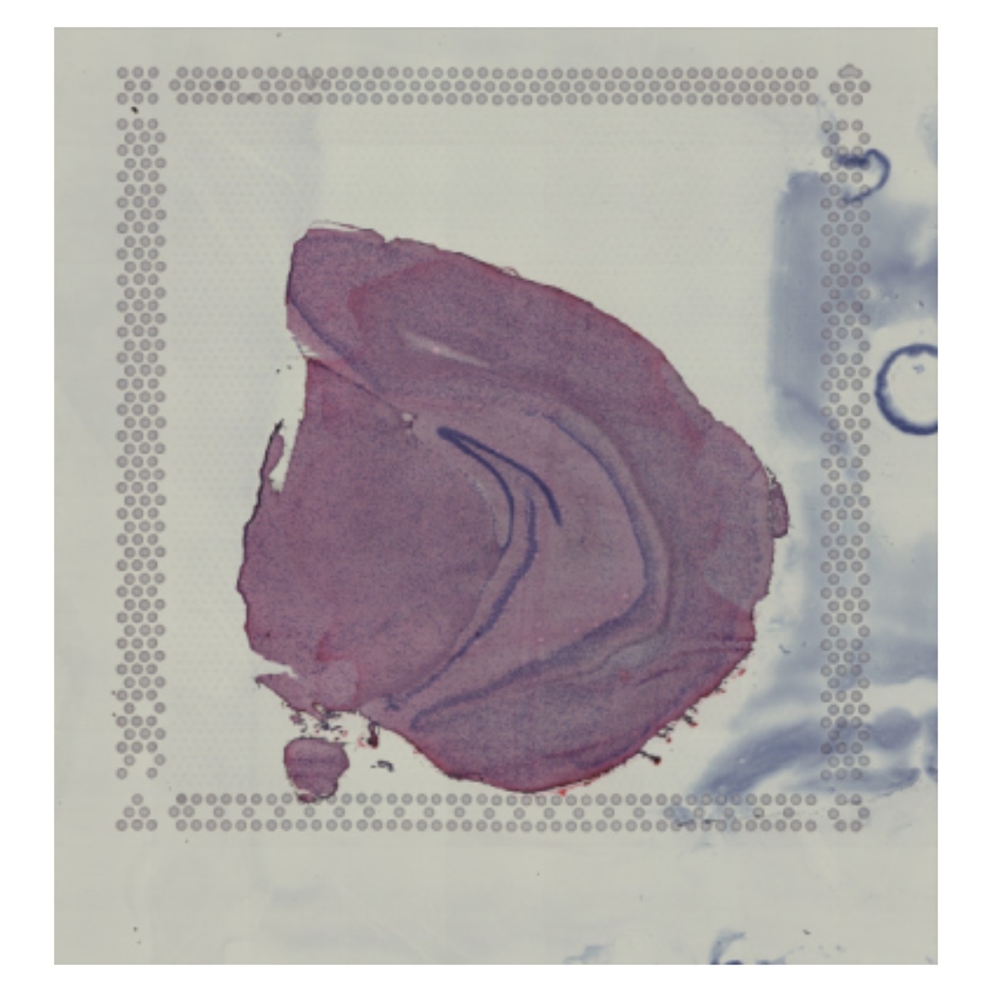
semla offers two ways of manipulating the orientation
and position of H&E images using rigid transformations. Allowed
transformations are:
- translation => move H&E image along x- and/or y-axis
- rotation => rotate image by a fixed degree
- mirror => mirror H&E image along x- and/or y-axis
Transformations can be applied to the H&E images programatically or interactively:
-
RigidTranformImages(): if you know what transformations to apply -
RunAlignment(): opens an interactive viewer where you can manipulate the H&E images
Basic image transformation
The first step is to generate a tibble with the transformations that
you want to apply. generate_rigid_transform() is a helper
function that makes this task a bit easier.
In the example below, we’ll mirror the H&E image along the x
axis, rotate it by 30 degrees, move it 20% to the right and 20% up.
Translations (tr_x and tr_y) are provided as
proportions. For example, tr_x = 0.1 means that you’ll move
the H&E image 20% of the image width to the right.
transforms <- generate_rigid_transform(mirror_x = TRUE, angle = 30, tr_x = 0.2, tr_y = -0.2)
transforms
## # A tibble: 1 × 7
## sampleID mirror_x mirror_y angle tr_x tr_y scalefactor
## <dbl> <lgl> <lgl> <dbl> <dbl> <dbl> <dbl>
## 1 1 TRUE FALSE 30 0.2 -0.2 1Now we are ready to apply the transformations:
se_mbrain <- RigidTransformImages(se_mbrain, transforms = transforms)The original H&E image is still stored in the Seurat
object, so when plotting we need to specify that we want to use the
transformed image:
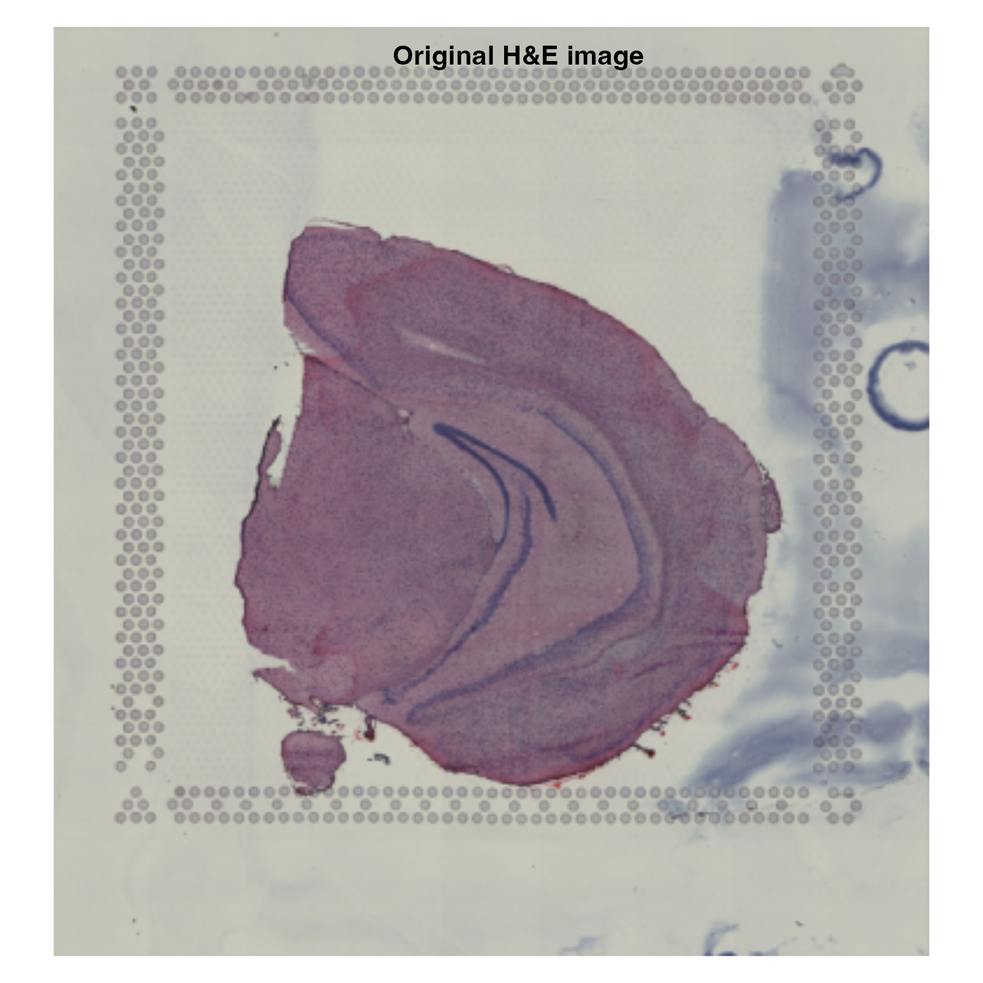
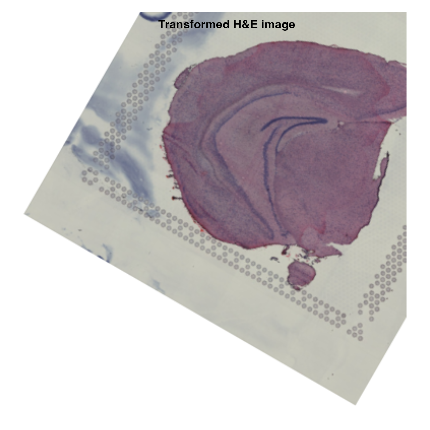
The spot coordinates are transformed together with the H&E image,
so if we use MapFeatures() or MapLabels(), we
should see that the spots are still correctly positioned on the H&E
image.
NB: Translations might result in moving parts of the H&E image outside of the predefined ‘canvas’. In our example below, this results in some spots being located outside of the view and these will therefore be dropped. The original image dimensions are always retained.
MapFeatures(se_mbrain, features = "nFeature_Spatial", image_use = "transformed")## Warning: Removed 27 rows containing missing values or values outside the scale range
## (`geom_point()`).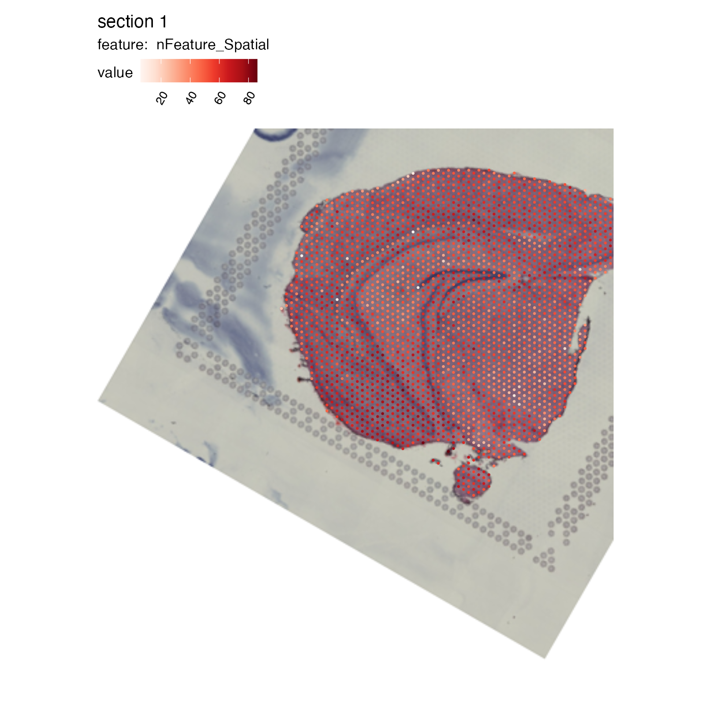
Interactive alignment
Here we will take a look at three H&E images with different orientations, and the goal is to align them to a common coordinate system.
You can click on ‘show’ to see the code used to generate this dummy
data using RigidTransformImages.
show
se_merged <- MergeSTData(se_mbrain, list(se_mbrain, se_mbrain)) |> LoadImages()
transforms1 <- generate_rigid_transform(mirror_x = TRUE, angle = 45, sampleID = 1)
transforms2 <- generate_rigid_transform(mirror_x = TRUE, scalefactor = 0.8, sampleID = 2)
transforms3 <- generate_rigid_transform(mirror_y = TRUE, scalefactor = 0.6, sampleID = 3)
transforms <- bind_rows(transforms1, transforms2, transforms3)
se_merged <- RigidTransformImages(se_merged, transforms = transforms, verbose = TRUE)
se_merged@tools$Staffli@rasterlists$raw <- se_merged@tools$Staffli@rasterlists$transformed
se_merged@tools$Staffli@rasterlists$transformed <- NULL
se_merged@tools$Staffli@meta_data <- se_merged@tools$Staffli@meta_data |>
  select(-pxl_col_in_fullres, -pxl_row_in_fullres) |>
  rename(pxl_col_in_fullres = pxl_col_in_fullres_transformed, pxl_row_in_fullres = pxl_row_in_fullres_transformed)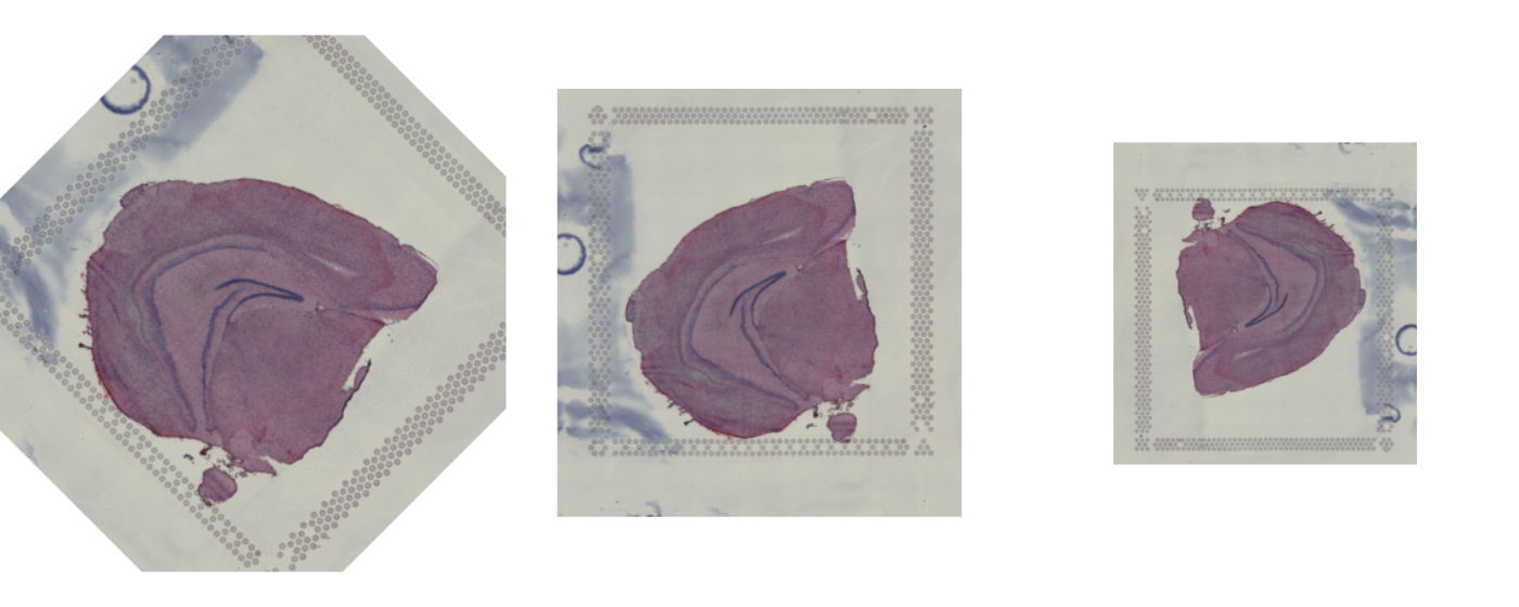
se_merged <- RunAlignment(se_merged)When we call RunAlignment, an interactive application
will open up in a separate window.
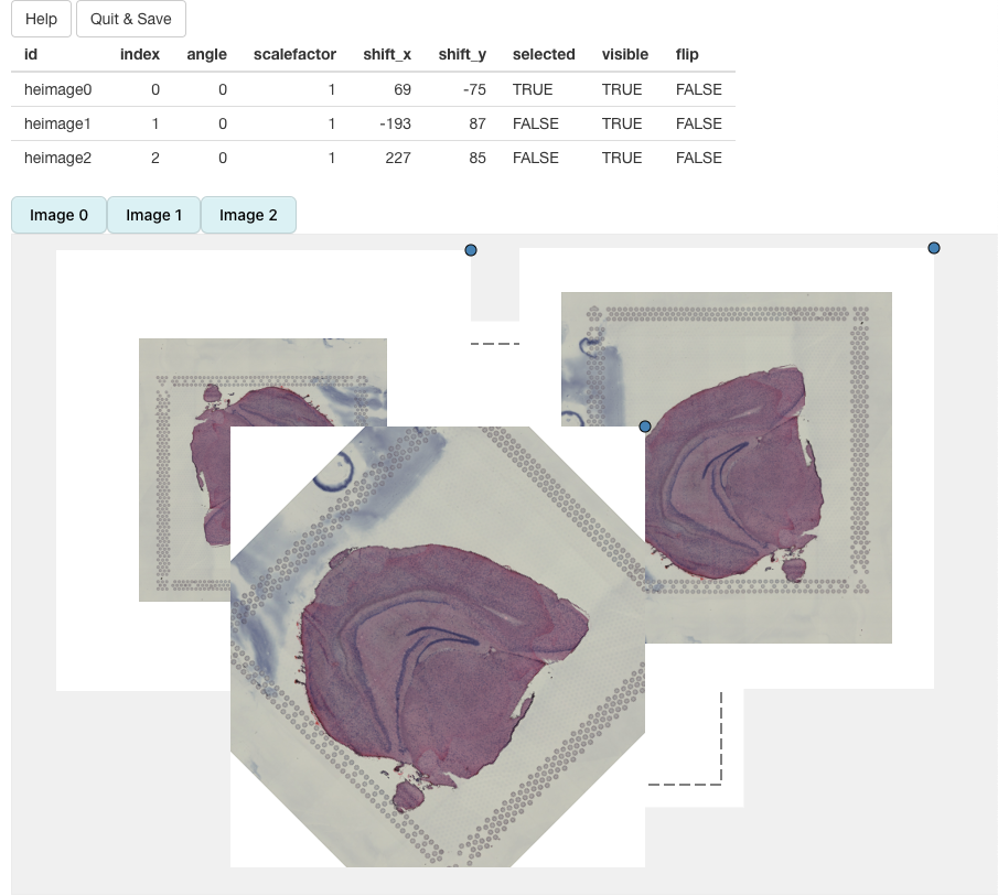
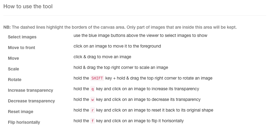
If you click on Help, you will see instructions on how
to use the app:
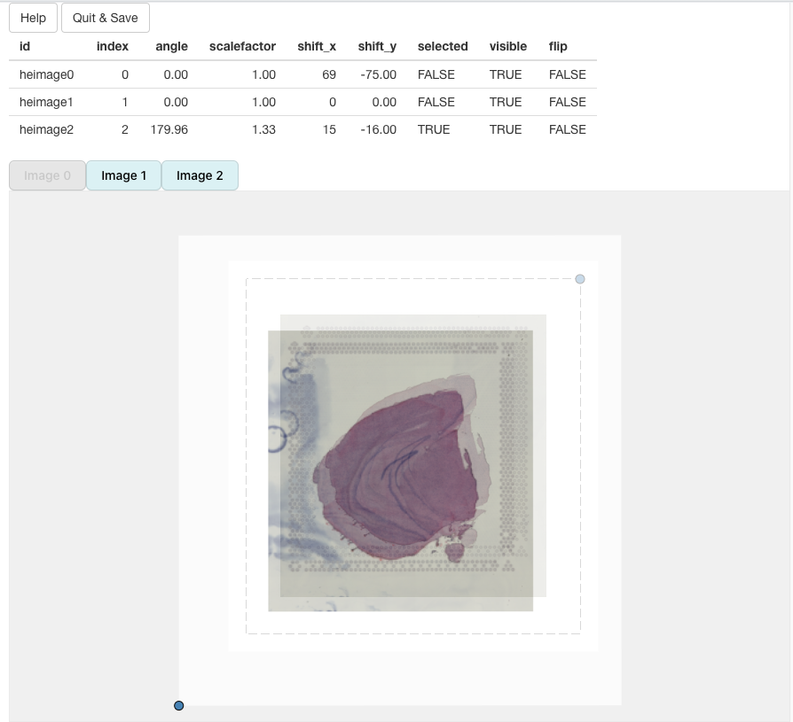
We can select what H&E images should be put into view by clicking on the button above the alignment panel:
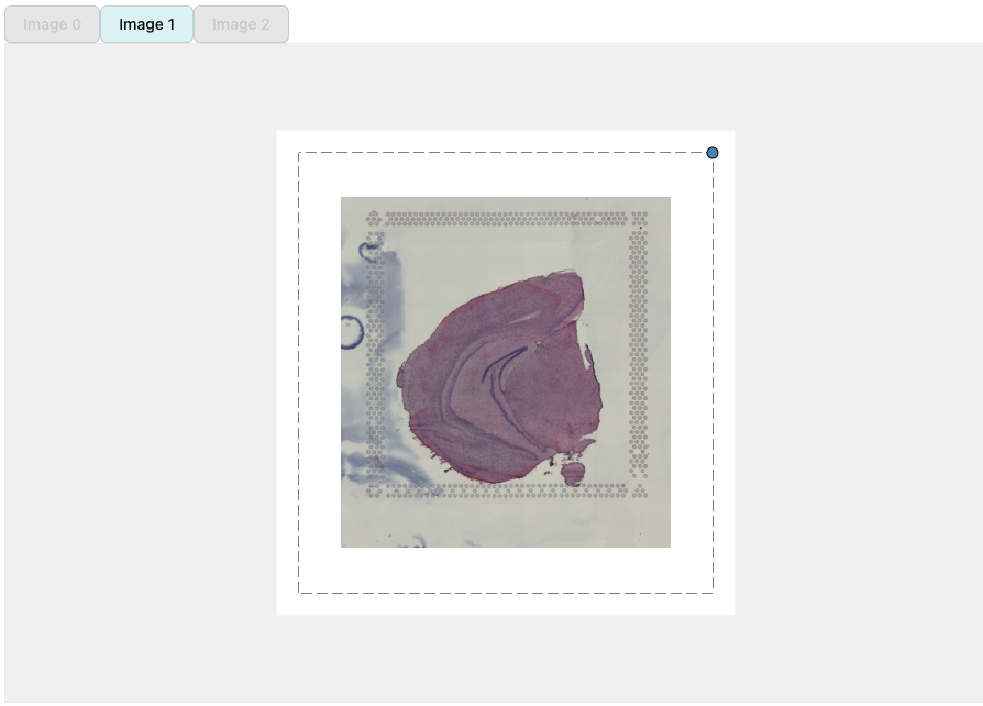
H&E images can be moved around by dragging the image with the cursor. The dotted borders around the H&E images highlights the dimensions of the ‘canvas’. Anything outside of these borders will be removed.
Some of the interaction is handled by pressing a key and clicking on
an H&E image. For example, you can change the transparency by
holding q or w and clicking on an H&E
image.
We can rotate an H&E image by holding SHIFT and
dragging the blue dot in the corner of the image. Similarly, scaling can
be done by holding and dragging the blue dot.
In the example below, we can see that ‘image2’ has been scaled and rotated to align with ‘image1’. All that is left is align ‘image2’ with ‘image1’:
In the end, we should be able to get a decent alignment of the three H&E images. The table on top of the alignment panel shows the transformations that have been applied:
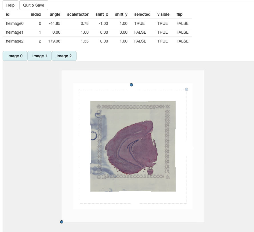
Once we are satisfied with the alignment, we can press the
Quit & Save button which will trigger the alignment of
our H&E images (in R) and the results will be saved to our
Seurat object.
If we set image_use='transformed' in
MapFeatures, we will see that the the H&E images are
now aligned.
NB: Manipulating the images will often lead to some cropping. In the first image below, we can see that the corners are cropped and filled with empty white space.
MapFeatures(se_merged, features = "nFeature_Spatial", image_use = "transformed", ncol = 3) &
  theme(legend.position = "right", legend.text = element_text(angle = 0))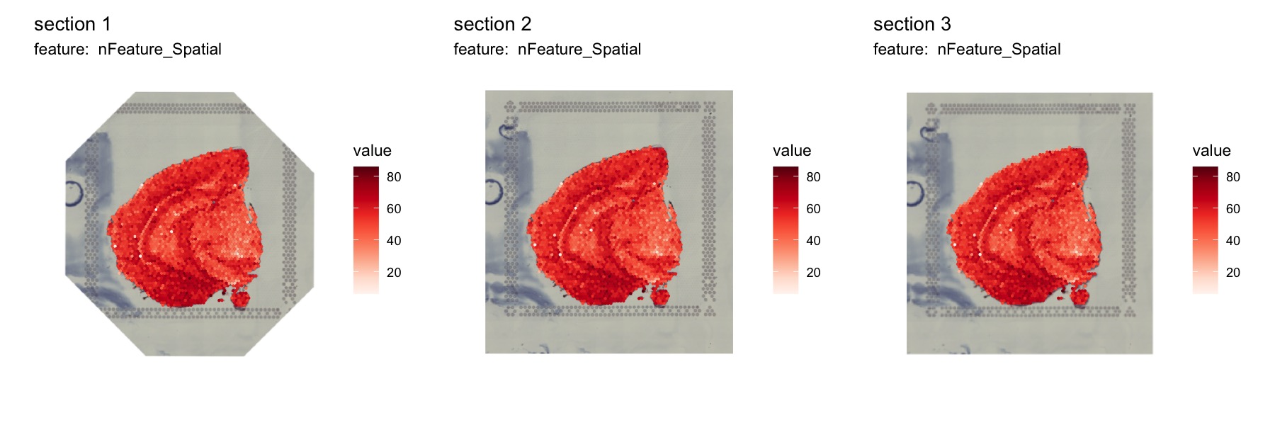
Now that the data is aligned, it will be easier to look at specific
areas of the tissue sections with the crop_area option
se_merged <- LoadImages(se_merged, image_height = 1.5e3)
MapFeatures(se_merged, features = "nFeature_Spatial", image_use = "transformed",
            ncol = 3, crop_area = c(0.4, 0.43, 0.6, 0.67)) &
  theme(legend.position = "right", legend.text = element_text(angle = 0))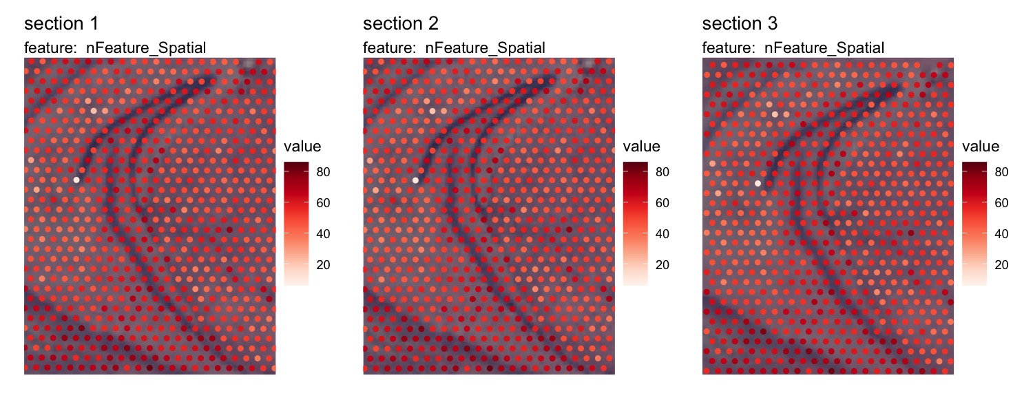
Images with different dimensions
RunAlignment applies the transformations to each image
independently and makes sure that the original dimensions of the images
are kept. This behavior might seem confusing at first. Let’s say that
you want to force all images to align with the first H&E image so
that you can use the transformed coordinates for 3D visualization, this
will not work without some additional processing.
In the example below, we can see two H&E images with slightly different dimensions. The second image (mouse colon tissue) has an aspect ration lower than 1 whereas the first image (mouse brain tissue) has an aspect ratio higher than 1 but both images are loaded with the same height. When applying transformations to the second image, the dashed box will only define where the image will be placed relative to the first image, but the image will keep its aspect ratio.
se_mbrain <- readRDS(file = system.file("extdata",
"mousebrain/se_mbrain",
package = "semla"))
se_mcolon <- readRDS(file = system.file("extdata",
"mousecolon/se_mcolon",
package = "semla"))
se_merged <- MergeSTData(se_mbrain, se_mcolon) |> LoadImages()
se_merged <- RunAlignment(se_merged)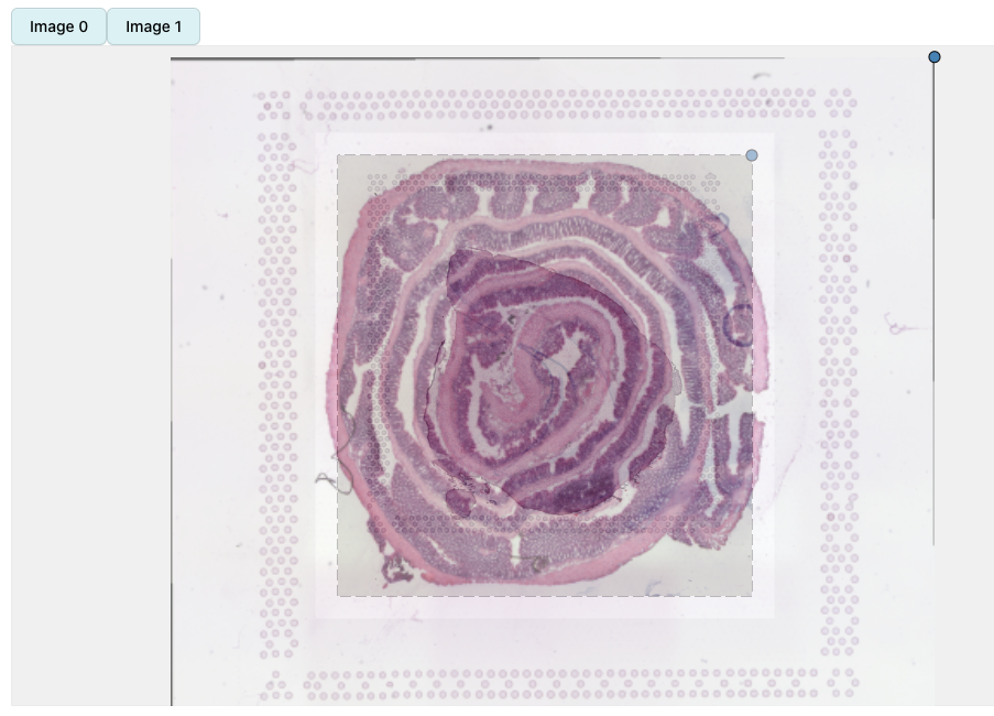 If we
apply rigid transformations according to the image above, the result
will be this:
ImagePlot(se_merged, image_use = "transformed")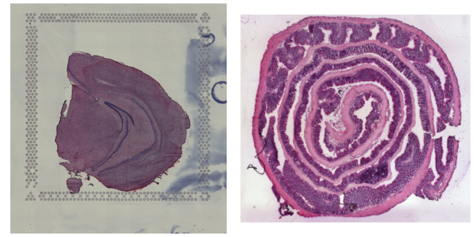
Here you can see that the second image fits the top and bottom of the dashed box, but the sides are wider than the box.
3D visualization
3D visualization requires some additional processing. For each tissue section, the spot coordinates can be defined on completely different scales. In order to place the coordinates on the same scale, we can adjust the coordinates by dividing them with the width/height of the H&E images.
The code below can be used to scale the transformed coordinates to a
common coordinate system, in this case they will range from 0 to 1. We
can use the sampleID as a z-coordinate to create a
“z-stack” that can be visualized in 3D.
Below is a simple example showing how to plot sots from stacked and aligned tissue sections in 3D using the plotly R package. In the example we are just stacking three identical tissue sections, so we can use the default coordinates for the visualization.
# Merge data from three identical objects for the demo
se_merged <- MergeSTData(se_mbrain, list(se_mbrain, se_mbrain))

xy_coords <- GetCoordinates(se_merged) |>
  # Note that we use pxl_*_in_fullres here. If ypu have aligned sections, use
  # pxl_*_in_fullres_transformed instead
  select(pxl_col_in_fullres, pxl_row_in_fullres, sampleID) |>
  group_by(sampleID) |>
  group_split()

image_info <- GetImageInfo(se_merged)

# Adjust coordinates
adjusted_coords <- do.call(bind_rows, lapply(seq_along(xy_coords), function(i) {
  xy <- xy_coords[[i]]
  full_width <- image_info[i, ]$full_width
  full_height <- image_info[i, ]$full_height
  xy <- xy |>
    mutate(x = pxl_col_in_fullres/full_width,
           y = pxl_row_in_fullres/full_height) |>
    # Here we can use the sampleID to define a z value.
    # We can also adjust it appropriately to set the distance between the sections.
    mutate(z = sampleID*0.2) |>
    select(x, y, z)
}))

# Obtain clusters for visualization
se_merged <- se_merged |>
  FindVariableFeatures() |>
  ScaleData() |>
  RunPCA() |>
  FindNeighbors() |>
  FindClusters(vresolution = 0.4)
## Modularity Optimizer version 1.3.0 by Ludo Waltman and Nees Jan van Eck
##
## Number of nodes: 7680
## Number of edges: 318594
##
## Running Louvain algorithm...
## Maximum modularity in 10 random starts: 0.8363
## Number of communities: 15
## Elapsed time: 0 seconds
# 3D scatter plot with plotly
library(plotly)
plot_ly(adjusted_coords, x = ~x, y = ~y, z = ~z, type = "scatter3d", mode = "markers", color = se_merged$seurat_clusters, size = 1)
Package version
-
semla: 1.4.1
Session info
## R version 4.4.2 (2024-10-31)
## Platform: aarch64-apple-darwin20.0.0
## Running under: macOS Sequoia 15.7.3
##
## Matrix products: default
## BLAS/LAPACK: /Users/javierescudero/miniconda3/envs/r-semlaupd/lib/libopenblas.0.dylib;  LAPACK version 3.12.0
##
## locale:
## [1] en_US.UTF-8/en_US.UTF-8/en_US.UTF-8/C/en_US.UTF-8/en_US.UTF-8
##
## time zone: Europe/Stockholm
## tzcode source: system (macOS)
##
## attached base packages:
## [1] stats     graphics  grDevices utils     datasets  methods   base
##
## other attached packages:
## [1] plotly_4.11.0      semla_1.4.1        ggplot2_3.5.2      dplyr_1.1.4
## [5] Seurat_5.3.0       SeuratObject_5.1.0 sp_2.2-0
##
## loaded via a namespace (and not attached):
##   [1] RColorBrewer_1.1-3     rstudioapi_0.17.1      jsonlite_1.9.0
##   [4] magrittr_2.0.3         spatstat.utils_3.1-4   magick_2.8.7
##   [7] farver_2.1.2           rmarkdown_2.29         fs_1.6.5
##  [10] ragg_1.3.3             vctrs_0.6.5            ROCR_1.0-11
##  [13] spatstat.explore_3.4-3 htmltools_0.5.8.1      forcats_1.0.0
##  [16] sass_0.4.9             sctransform_0.4.2      parallelly_1.42.0
##  [19] KernSmooth_2.23-26     bslib_0.9.0            htmlwidgets_1.6.4
##  [22] desc_1.4.3             ica_1.0-3              plyr_1.8.9
##  [25] zoo_1.8-13             cachem_1.1.0           igraph_2.1.4
##  [28] mime_0.12              lifecycle_1.0.4        pkgconfig_2.0.3
##  [31] Matrix_1.7-2           R6_2.6.1               fastmap_1.2.0
##  [34] fitdistrplus_1.2-3     future_1.34.0          shiny_1.10.0
##  [37] digest_0.6.37          colorspace_2.1-1       patchwork_1.3.1
##  [40] tensor_1.5.1           RSpectra_0.16-2        irlba_2.3.5.1
##  [43] crosstalk_1.2.1        textshaping_0.4.0      labeling_0.4.3
##  [46] progressr_0.15.1       spatstat.sparse_3.1-0  httr_1.4.7
##  [49] polyclip_1.10-7        abind_1.4-5            compiler_4.4.2
##  [52] withr_3.0.2            fastDummies_1.7.5      MASS_7.3-64
##  [55] tools_4.4.2            lmtest_0.9-40          httpuv_1.6.15
##  [58] future.apply_1.11.3    goftest_1.2-3          glue_1.8.0
##  [61] dbscan_1.2.2           nlme_3.1-167           promises_1.3.2
##  [64] grid_4.4.2             Rtsne_0.17             cluster_2.1.8
##  [67] reshape2_1.4.4         generics_0.1.3         gtable_0.3.6
##  [70] spatstat.data_3.1-6    tidyr_1.3.1            data.table_1.17.0
##  [73] spatstat.geom_3.4-1    RcppAnnoy_0.0.22       ggrepel_0.9.6
##  [76] RANN_2.6.2             pillar_1.10.1          stringr_1.5.1
##  [79] spam_2.11-1            RcppHNSW_0.6.0         later_1.4.1
##  [82] splines_4.4.2          lattice_0.22-6         survival_3.8-3
##  [85] deldir_2.0-4           tidyselect_1.2.1       miniUI_0.1.1.1
##  [88] pbapply_1.7-2          knitr_1.50             gridExtra_2.3
##  [91] scattermore_1.2        xfun_0.53              matrixStats_1.5.0
##  [94] stringi_1.8.4          lazyeval_0.2.2         yaml_2.3.10
##  [97] evaluate_1.0.5         codetools_0.2-20       tibble_3.2.1
## [100] cli_3.6.4              uwot_0.2.3             xtable_1.8-4
## [103] reticulate_1.42.0      systemfonts_1.3.1      munsell_0.5.1
## [106] jquerylib_0.1.4        Rcpp_1.1.0             globals_0.16.3
## [109] spatstat.random_3.4-1  zeallot_0.2.0          png_0.1-8
## [112] spatstat.univar_3.1-3  parallel_4.4.2         pkgdown_2.1.1
## [115] dotCall64_1.2          listenv_0.9.1          viridisLite_0.4.2
## [118] scales_1.3.0           ggridges_0.5.6         purrr_1.0.4
## [121] rlang_1.1.5            cowplot_1.1.3          shinyjs_2.1.0