Map categorical features
visualize-labels.RdMapLabels colors spots based on the values of a categorical feature.
Usage
MapLabels(object, ...)

# Default S3 method
MapLabels(
  object,
  spot_side = NULL,
  crop_area = NULL,
  pt_size = 1,
  pt_alpha = 1,
  pt_stroke = 0,
  shape = "point",
  section_number = NULL,
  label_by = NULL,
  split_labels = FALSE,
  ncol = NULL,
  colors = NULL,
  dims = NULL,
  coords_columns = c("pxl_col_in_fullres", "pxl_row_in_fullres"),
  return_plot_list = FALSE,
  drop_na = FALSE,
  add_scalebar = FALSE,
  scalebar_gg = NULL,
  scalebar_height = 0.05,
  scalebar_position = c(0.8, 0.8),
  ...
)

# S3 method for class 'Seurat'
MapLabels(
  object,
  column_name,
  image_use = NULL,
  coords_use = "raw",
  crop_area = NULL,
  pt_size = 1,
  pt_alpha = 1,
  pt_stroke = 0,
  shape = "point",
  spot_side = NULL,
  section_number = NULL,
  label_by = NULL,
  split_labels = FALSE,
  ncol = NULL,
  colors = NULL,
  override_plot_dims = FALSE,
  return_plot_list = FALSE,
  drop_na = FALSE,
  add_scalebar = FALSE,
  scalebar_height = 0.05,
  scalebar_gg = scalebar(x = 500, text_height = 5),
  scalebar_position = c(0.8, 0.7),
  ...
)
Arguments
- object
An object
- ...
Arguments passed to other methods
- spot_side
A numeric value or vector of values specifying the size of the spots in pixels in the fullres image. Relevant for tile shape. Will default to each section's value retrieved via GetScaleFactors:
GetScaleFactors()$spot_diameter_fullres).- crop_area
A numeric vector of length 4 specifying a rectangular area to crop the plots by. These numbers should be within 0-1. The x-axis is goes from left=0 to right=1 and the y axis is goes from top=0 to bottom=1. The order of the values are specified as follows:
crop_area = c(left, top, right, bottom). The crop area will be used on all tissue sections and cannot be set for each section individually. using crop areas of different sizes on different sections can lead to unwanted side effects as the point sizes will remain constant. In this case it is better to generate separate plots for different tissue sections.- pt_size
A numeric value specifying the point size passed to
geom_point- pt_alpha
A numeric value between 0 and 1 specifying the point opacity passed to
geom_point. A value of 0 will make the points completely transparent and a value of 1 will make the points completely opaque.- pt_stroke
A numeric specifying the point stroke width
- shape
A string specifying the shape to plot. Options are:
c("point", "raster", "tile").- section_number
An integer select a tissue section number to subset data by
- label_by
A character specifying a column name in
objectwith labels that can be used to provide a title for each subplot. This column should have 1 label per tissue section. This can be useful when you need to provide more detailed information about your tissue sections.- split_labels
A logical specifying if labels should be split.
- ncol
An integer value specifying the number of columns in the output patchwork.
- colors
A character vector of colors to use for the color scale. The number of colors should match the number of labels present.
- dims
A tibble with information about the tissue sections. This information is used to determine the limits of the plot area. If
dimsis not provided, the limits will be computed directly from the spatial coordinates provided inobject.- coords_columns
A character vector of length 2 specifying the names of the columns in
objectholding the spatial coordinates- return_plot_list
logical specifying whether the plots should be return as a list of
ggplotobjects. Ifreturn_plot_list = FALSE(default), the plots will be arranged into apatchwork- drop_na
A logical specifying if NA values should be dropped
- add_scalebar
A logical specifying if a scale bar should be added to the plots
- scalebar_gg
A 'ggplot' object generated with
scalebar. The appearance of the scale bar is styled by passing parameters toscalebar.- scalebar_height
A numeric value specifying the height of the scale bar relative to the height of the full plot area. Has to be a value between 0 and 1. The title of the scale bar is scaled with the plot and might disappear if the down-scaled text size is too small. Increasing the height of the scale bar can sometimes be useful to increase the text size to make it more visible in small plots.
- scalebar_position
A numeric vector of length 2 specifying the position of the scale bar relative to the plot area. Default is to place it in the top right corner.
- column_name
A character specifying a meta data column holding the categorical feature vector.
- image_use
A character specifying image type to use.
- coords_use
A character specifying coordinate type to use.
- override_plot_dims
A logical specifying whether the image dimensions should be used to define the plot area. Setting
override_plot_dimscan be useful in situations where the tissue section only covers a small fraction of the capture area, which will create a lot of white space in the plots. The same effect can be achieved with thecrop_areabut the crop area is instead determined directly from the data.
Details
You can only plot categorical features with MapLabels,
for example: spot annotations or clusters.
If you want to plot numerical features, use MapFeatures instead.
Only 1 categorical feature can be provided.
See also
Other spatial-visualization-methods:
AnglePlot(),
FeatureViewer(),
ImagePlot(),
MapFeatures(),
MapFeaturesSummary(),
MapLabelsSummary(),
MapMultipleFeatures()
Examples
library(semla)
# Load Seurat object
se_mbrain <- readRDS(system.file("extdata/mousebrain", "se_mbrain", package = "semla"))
# Run PCA and data-driven clustering
se_mbrain <- se_mbrain |>
ScaleData() |>
RunPCA() |>
FindNeighbors(reduction = "pca", dims = 1:10) |>
FindClusters(resolution = 0.2) |>
FindClusters(resolution = 0.3)
#> Centering and scaling data matrix
#> PC_ 1
#> Positive: Nrgn, Olfm1, Cck, Nptxr, Rtn1, Snca, Nov, Tmsb4x, Lamp5, Egr1
#> Crym, Cpne6, Coro1a, Arc, Hpca, Sst, Nr4a1, Npy, Chgb, Neurod6
#> Snap25, Myh7, Uchl1, Eef1a2, Cort, Grp, Stmn2, Rprm, Spink8, Mfge8
#> Negative: Mbp, Plp1, Apod, Mobp, Ptgds, Mog, Mal, Mag, Cnp, Aldh1a1
#> Opalin, Tcf7l2, Ddc, Lhx1os, Slc6a3, Ret, Th, Slc18a2, Sncg, Drd2
#> Chrna6, Slc10a4, Spp1, En1, Dlk1, Calb2, Hbb-bs, Pvalb, Col1a2, Tnnt1
#> PC_ 2
#> Positive: Myoc, Gfap, Col1a2, Fmod, Slc13a4, Hba-a1, Hbb-bt, Slc6a20a, Hba-a2, Hbb-bs
#> Acta2, Tagln, Mgp, Ogn, Vtn, H2-Aa, Lyz2, Cd74, Myl9, Dcn
#> Myh11, Ptgds, Cytl1, H2-Eb1, Hmgcs2, Clu, Mfge8, Emp1, Npy, Cnn1
#> Negative: Th, Uchl1, Slc18a2, En1, Slc10a4, Slc6a3, Chrna6, Stmn2, Ret, Snap25
#> Drd2, Dlk1, Ddc, Scg2, Sncg, Eef1a2, Rtn1, Chga, Pcp4, Calb2
#> Mobp, Mbp, Chgb, Fabp5, Plp1, Pvalb, Mog, Mal, Mag, Snca
#> PC_ 3
#> Positive: Trbc2, Arc, Egr1, Myl4, Nr4a1, Mbp, Mobp, Pvalb, Plp1, Opalin
#> Mog, Mal, Cnp, Mag, Snap25, Lamp5, Ighm, Tcf7l2, Cplx3, Tgm3
#> Ighg2c, Pcp4, Hpca, Ly6d, Eef1a2, Tnnt1, Chga, Neurod6, Prph, Ctgf
#> Negative: Nnat, Slc18a2, Dlk1, Slc6a3, Slc10a4, En1, Th, Chrna6, Dcn, Sncg
#> Cpne7, Drd2, Ddc, Ret, Hpcal1, Ecel1, Cpne6, Col1a2, Trh, Calb2
#> Cd24a, Fmod, Mgp, Snca, Lypd1, Slc13a4, Fibcd1, Crym, Spink8, Slc6a20a
#> PC_ 4
#> Positive: Nr4a1, Arc, Lamp5, Egr1, Myl4, Trbc2, Chrna6, Tagln, En1, Snap25
#> Th, Slc18a2, Acta2, Col1a2, Myh11, Fmod, Hba-a2, Slc10a4, Slc6a3, Slc13a4
#> Ret, Tgm3, Hbb-bt, Slc6a20a, Ighm, Hbb-bs, Hba-a1, Vtn, Mgp, Drd2
#> Negative: Spink8, Fibcd1, Tmsb4x, Nnat, Lefty1, Crym, Cpne7, Nos1, Dcn, Cpne6
#> Grp, Homer3, Htr3a, Tac1, Fabp5, C1ql2, Trh, Opalin, Mog, Plp1
#> Mag, Calb2, Ecel1, Gfap, Cnp, Tcf7l2, Lypd1, Vgll3, Hpcal1, Mal
#> PC_ 5
#> Positive: Pcp4, Tcf7l2, Snap25, Uchl1, Eef1a2, Chga, Stmn2, Lhx1os, Calb2, Scg2
#> Fabp5, Bok, Prkcd, Pvalb, Cartpt, Chgb, Tnnt1, Gpx3, Slc20a1, Rtn1
#> C1ql2, Spp1, Hpcal1, Ptgds, Pitx2, Lypd1, Aldh1a1, Ecel1, Vtn, Nme7
#> Negative: En1, Chrna6, Th, Slc18a2, Slc10a4, Ddc, Lefty1, Arc, Slc6a3, Neurod6
#> Grp, Nov, Lamp5, Fibcd1, Nr4a1, Drd2, Spink8, Vip, Myl4, Ret
#> Egr1, Dlk1, Nrgn, Gfap, Trbc2, Tgm3, Myh7, Tac2, Sncg, Npy
#> Computing nearest neighbor graph
#> Computing SNN
#> Modularity Optimizer version 1.3.0 by Ludo Waltman and Nees Jan van Eck
#>
#> Number of nodes: 2560
#> Number of edges: 85218
#>
#> Running Louvain algorithm...
#> Maximum modularity in 10 random starts: 0.9096
#> Number of communities: 6
#> Elapsed time: 0 seconds
#> Modularity Optimizer version 1.3.0 by Ludo Waltman and Nees Jan van Eck
#>
#> Number of nodes: 2560
#> Number of edges: 85218
#>
#> Running Louvain algorithm...
#> Maximum modularity in 10 random starts: 0.8881
#> Number of communities: 8
#> Elapsed time: 0 seconds
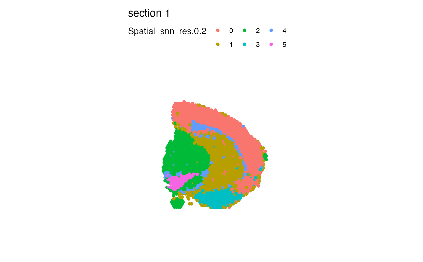
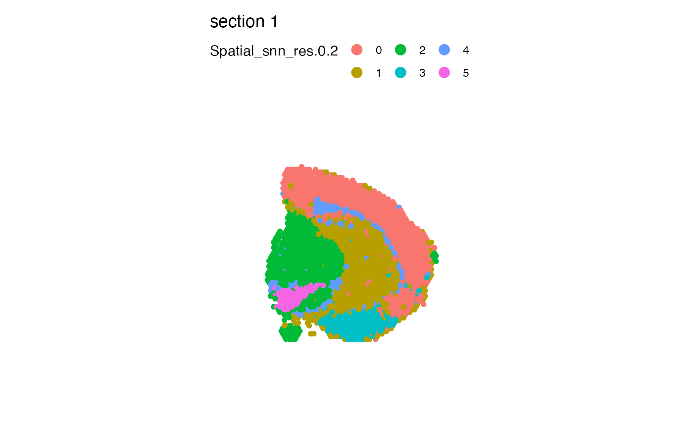
# Plot clusters
MapLabels(se_mbrain, column_name = "Spatial_snn_res.0.2", pt_size = 2)
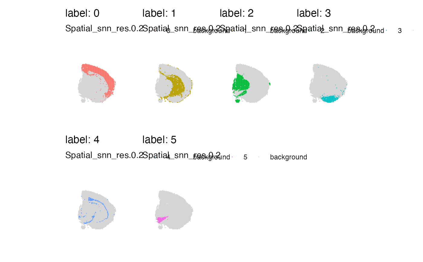
 # Plot clusters in split view
MapLabels(se_mbrain, column_name = "Spatial_snn_res.0.2", pt_size = 0.5,
section_number = 1, split_labels = TRUE, ncol = 4)
# Plot clusters in split view
MapLabels(se_mbrain, column_name = "Spatial_snn_res.0.2", pt_size = 0.5,
section_number = 1, split_labels = TRUE, ncol = 4)
 # \donttest{
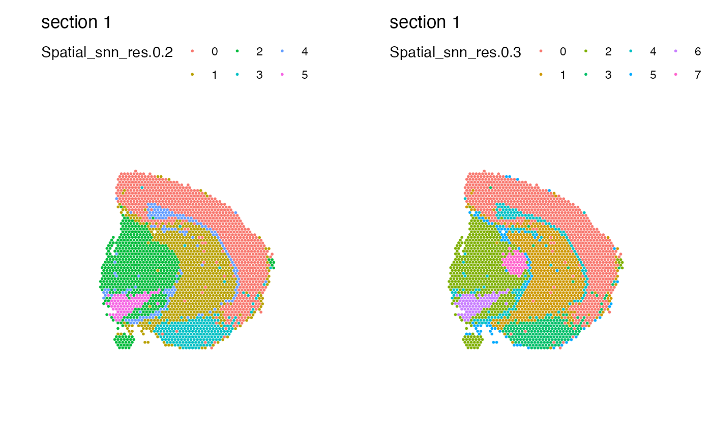
# Combine plots with different labels
MapLabels(se_mbrain, column_name = "Spatial_snn_res.0.2") |
MapLabels(se_mbrain, column_name = "Spatial_snn_res.0.3")
# \donttest{
# Combine plots with different labels
MapLabels(se_mbrain, column_name = "Spatial_snn_res.0.2") |
MapLabels(se_mbrain, column_name = "Spatial_snn_res.0.3")
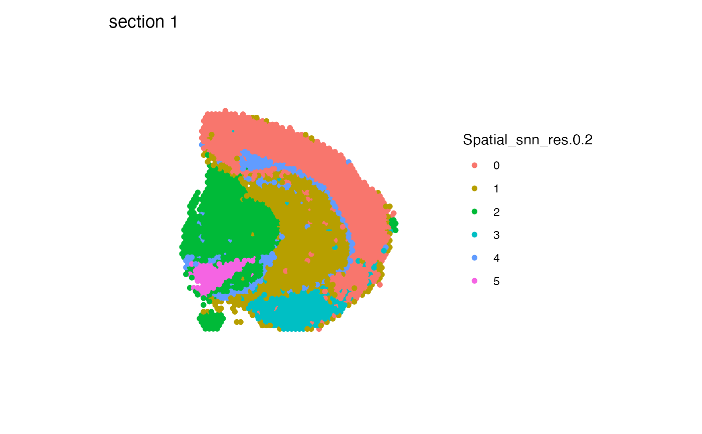
 # Move legend to the right side of the plot
MapLabels(se_mbrain, column_name = "Spatial_snn_res.0.2", pt_size = 2) &
theme(legend.position = "right")
# Move legend to the right side of the plot
MapLabels(se_mbrain, column_name = "Spatial_snn_res.0.2", pt_size = 2) &
theme(legend.position = "right")
 # Override fill aesthetic to increase point sixe in legend
MapLabels(se_mbrain, column_name = "Spatial_snn_res.0.2", pt_size = 2) &
guides(fill = guide_legend(override.aes = list(size = 4)))
# Override fill aesthetic to increase point sixe in legend
MapLabels(se_mbrain, column_name = "Spatial_snn_res.0.2", pt_size = 2) &
guides(fill = guide_legend(override.aes = list(size = 4)))
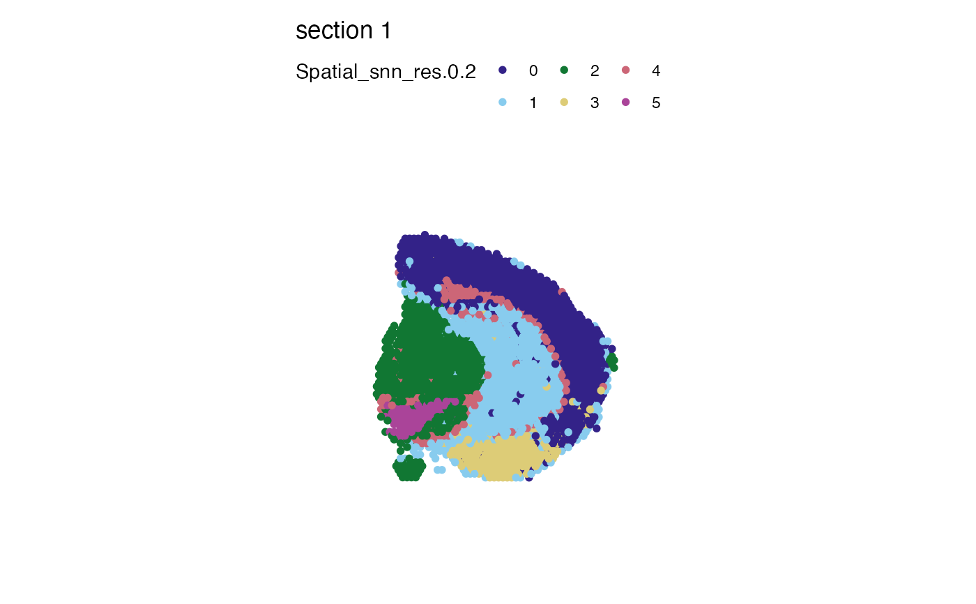
 # Use custom colors
cols <- c("#332288", "#88CCEE", "#117733", "#DDCC77", "#CC6677","#AA4499")
MapLabels(se_mbrain, column_name = "Spatial_snn_res.0.2", pt_size = 2, colors = cols)
# Use custom colors
cols <- c("#332288", "#88CCEE", "#117733", "#DDCC77", "#CC6677","#AA4499")
MapLabels(se_mbrain, column_name = "Spatial_snn_res.0.2", pt_size = 2, colors = cols)
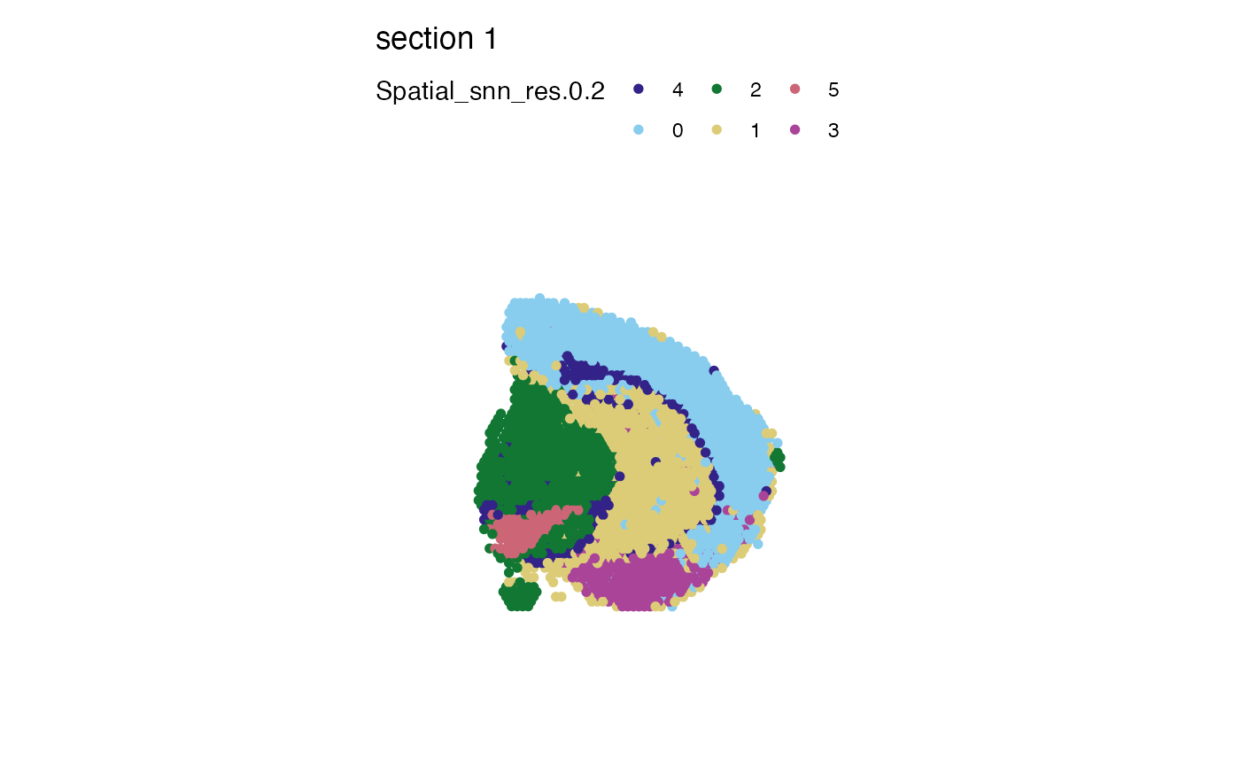
 # Factor are to used to determine the color order. If you change the
# levels of your label of interest, the labels and colors will change order
se_mbrain$Spatial_snn_res.0.2 <- factor(se_mbrain$Spatial_snn_res.0.2,
levels = sample(paste0(0:7), size = 8))
MapLabels(se_mbrain, column_name = "Spatial_snn_res.0.2", pt_size = 2, colors = cols)
# Factor are to used to determine the color order. If you change the
# levels of your label of interest, the labels and colors will change order
se_mbrain$Spatial_snn_res.0.2 <- factor(se_mbrain$Spatial_snn_res.0.2,
levels = sample(paste0(0:7), size = 8))
MapLabels(se_mbrain, column_name = "Spatial_snn_res.0.2", pt_size = 2, colors = cols)
 # Control what group label colors by naming the color vector
# this way you can make sure that each group gets a desired color
# regardless of the factor levels
cols <- setNames(cols, nm = paste0(0:5))
cols
#> 0 1 2 3 4 5
#> "#332288" "#88CCEE" "#117733" "#DDCC77" "#CC6677" "#AA4499"
MapLabels(se_mbrain, column_name = "Spatial_snn_res.0.2", pt_size = 2, colors = cols)
# Control what group label colors by naming the color vector
# this way you can make sure that each group gets a desired color
# regardless of the factor levels
cols <- setNames(cols, nm = paste0(0:5))
cols
#> 0 1 2 3 4 5
#> "#332288" "#88CCEE" "#117733" "#DDCC77" "#CC6677" "#AA4499"
MapLabels(se_mbrain, column_name = "Spatial_snn_res.0.2", pt_size = 2, colors = cols)
 # }
# }