Comparison of cell type mapping with NNLS
Last compiled: 20 March 2026
compare_cell_type_mapping_NNLS.RmdAs described in the tutorial Cell
type mapping with NNLS, there is an implementation of a cell type
mapping approach in semla based on the Non-Negative Least
Squares (NNLS) method, as implemented in the RcppML R package. Cell
type mapping algorithms utilizes a well annotated scRNA-seq data set to
learn cell type expression profiles in order to infer their relative
abundance or proportions onto the spatial data. In short, the approach
implemented in semla works by initially estimating
enrichment scores for each available cell type in the scRNA-seq data and
assigning weights to genes based on their cell type specificity. This
information is in the following steps leveraged in the NNLS methods to
solve the following optimization problem in order to assign cell type
composition predictions to each spatial coordinate in the Visium
data,
where A is a matrix with cell type enrichment scores, y is a vector with mixed a mixed gene expression profile. The solution for x represents estimates of the fractional abundances of cell type estimates.
To demonstrate the utility of this approach, we have performed a basic comparison with two other popular cell type mapping approaches, applied to two tissue types.
Cell type mapping methods
NNLS: Debruine, Zach & Melcher, Karsten & Triche, Timothy. (2021). Fast and robust non-negative matrix factorization for single-cell experiments. https://doi.org/10.1101/2021.09.01.458620
Stereoscope: Andersson, A., Bergenstråhle, J., Asp, M. et al. Single-cell and spatial transcriptomics enables probabilistic inference of cell type topography. Commun Biol 3, 565 (2020). https://doi.org/10.1038/s42003-020-01247-y
cell2location: Kleshchevnikov, V., Shmatko, A., Dann, E. et al. Cell2location maps fine-grained cell types in spatial transcriptomics. Nat Biotechnol 40, 661–671 (2022). https://doi.org/10.1038/s41587-021-01139-4
Data sets
-
Brain sagittal section (mouse).
scRNA-seq: Allen Brain, mouse atlas reference single cell RNA-seq data set
Visium: Mouse brain sagittal data (anterial + posterior) made available by 10x Genomics, processed using the Space Ranger pipeline v1.0.0
-
Kidney (mouse)
scRNA-seq: Tabula Muris Senis droplet data from kidney, made available by The Tabula Muris Consortium
Visium: Mouse kidney coronal section data made available by 10x Genomics, processed using the Space Ranger pipeline v1.1.0
The same Visium and reference scRNA-seq data sets were used as input for all cell type deconvolution methods tested. The code displayed in the Cell type mapping with NNLS vignette was used to produce the NNLS mapping results, while stereoscope and cell2location were run in python on high-performance computing servers using default parameter settings.
Mouse brain
The results of each cell type mapping approach is stored as an
Assay within the semla object, and the spot-wise
Pearson correlation values are computed using the cor()
function in R. The results are visualized as heatmaps using
ggplot2 and geom_tile(), where the fill color
corresponds to the strength of the correlation.
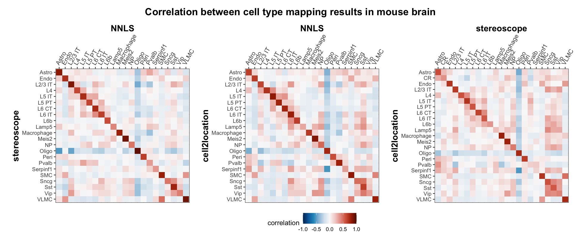
In general, we can see that the correlation between mapped cell types values is high between the NNLS method and the other two tested approaches. As we do not have any ground truth values, it is unfortunately impossible for us to tell which of these methods produce results closest to the true cell type proportions in each spot.
We can also summarize the results by looking at the correlation between matching cell types, to better view if the NNLS method seems to share a higher concordance with a specific method for certain cell types.
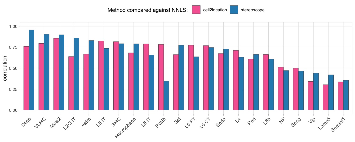
Here, we can for instance more easily spot a large difference in the correlation values between the NNLS:stereoscope an NNLS:cell2location for Pvalb cells, demonstrating an example of how different cell type mapping algorithms can perform drastically different despite the same input.
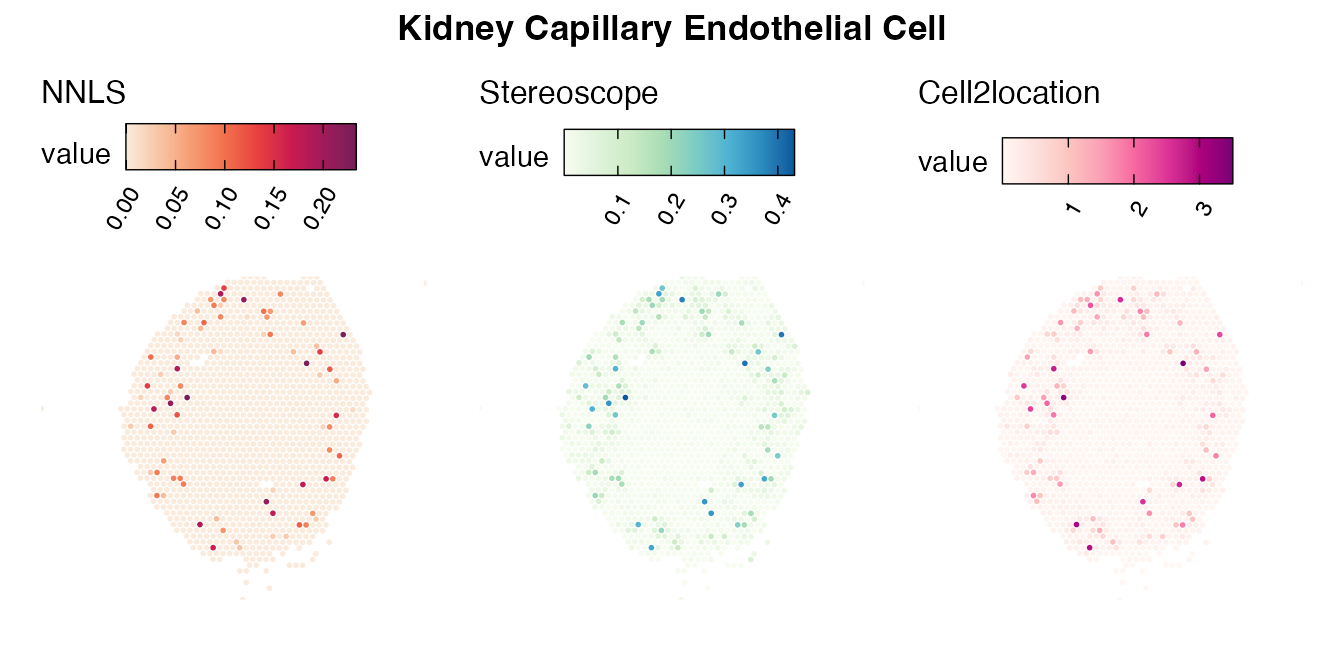
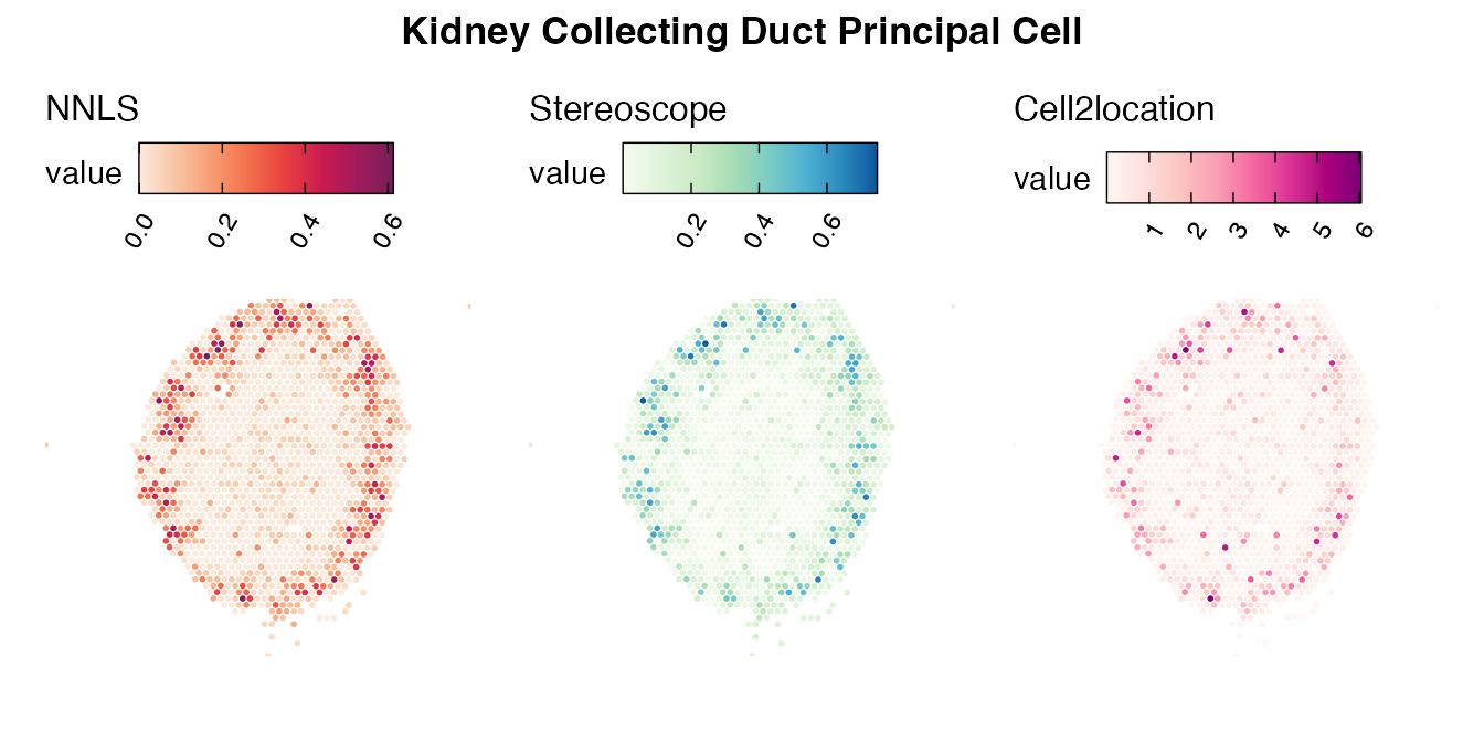
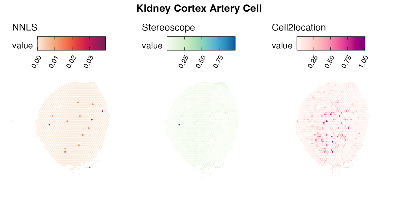
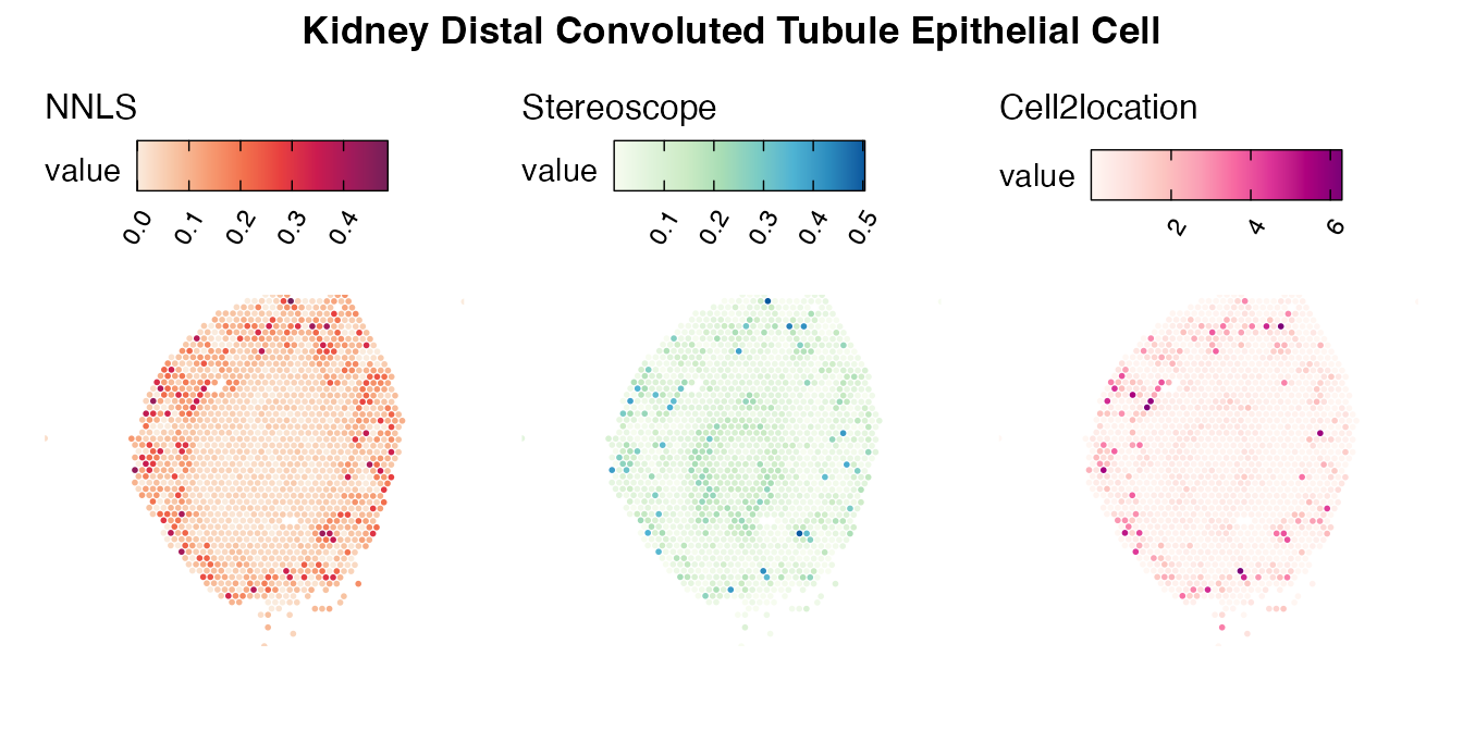
Lastly, let us have a look at the cell type mapping results from all three approaches spatially.
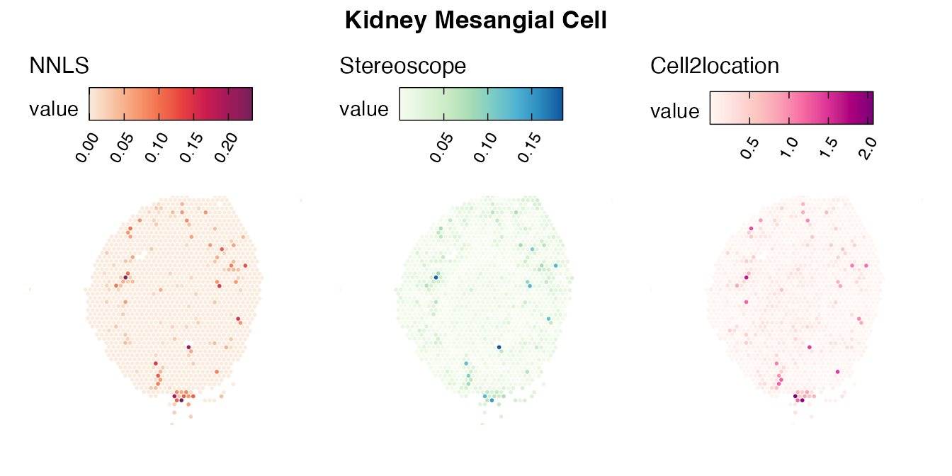
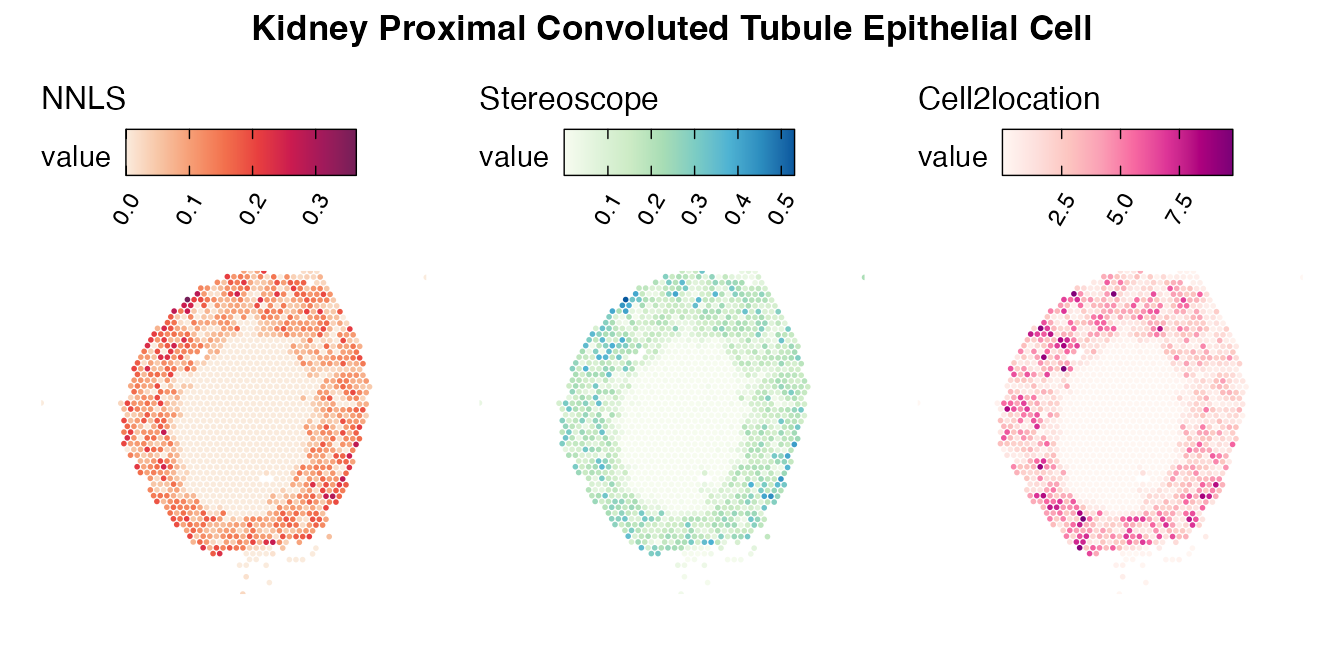
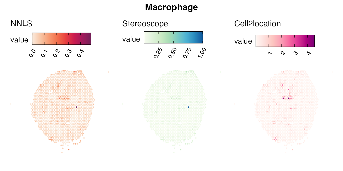
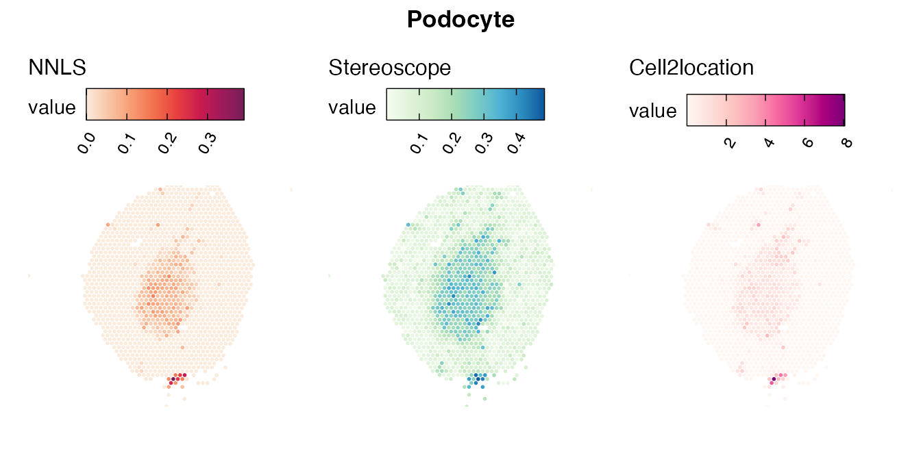
Mouse kidney
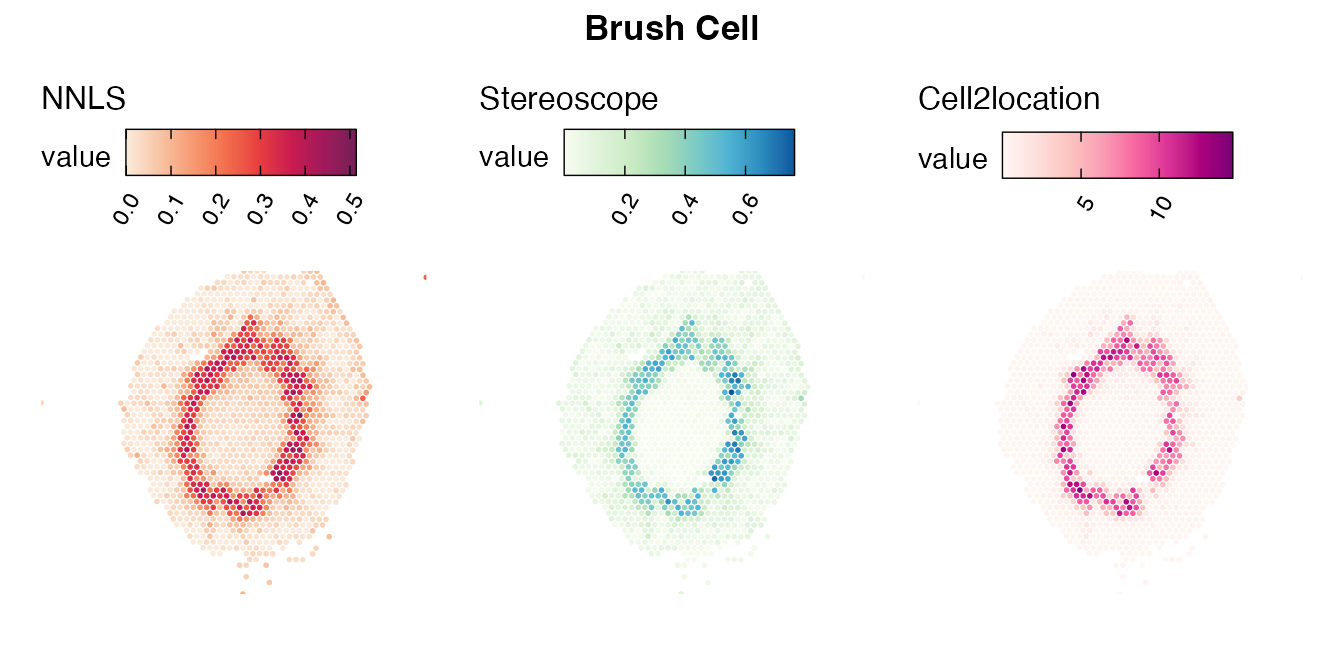
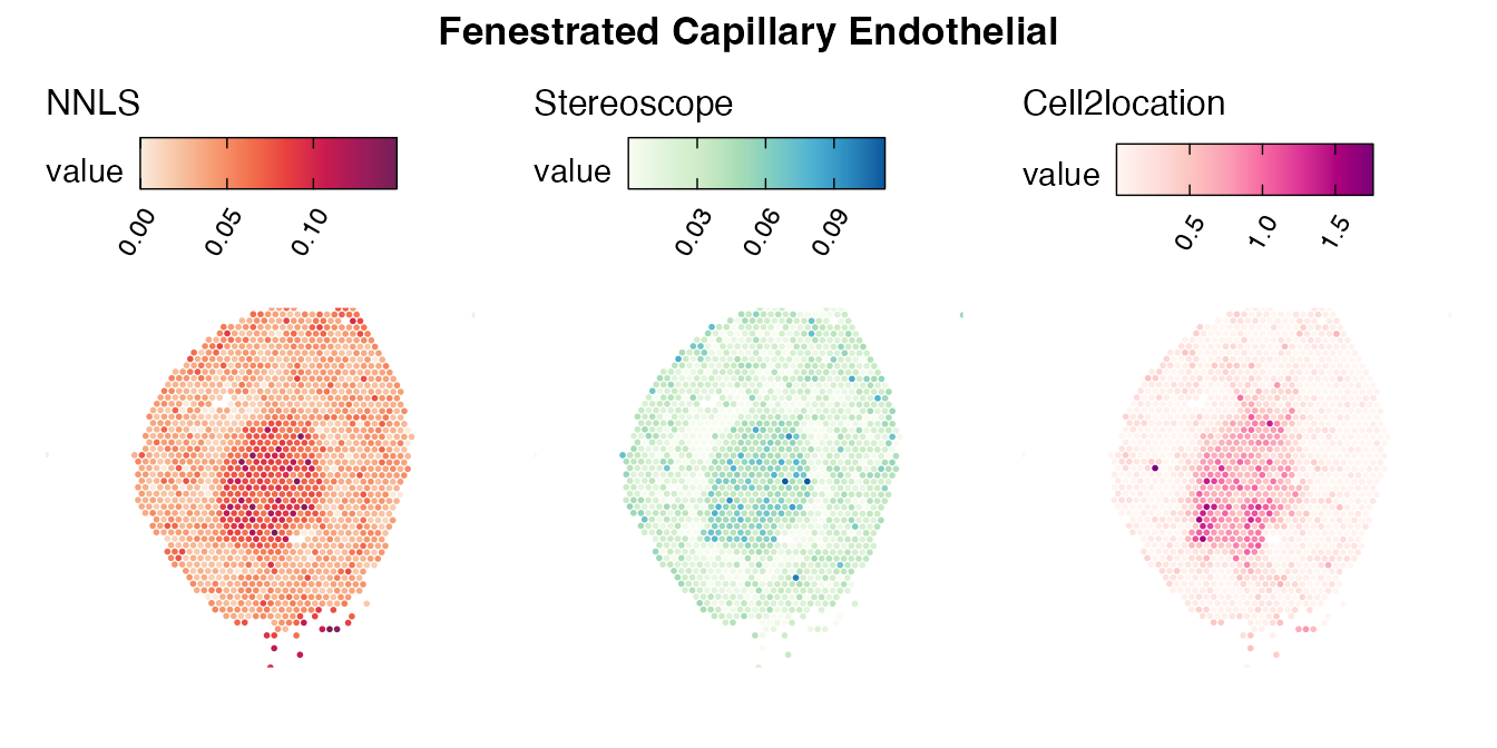
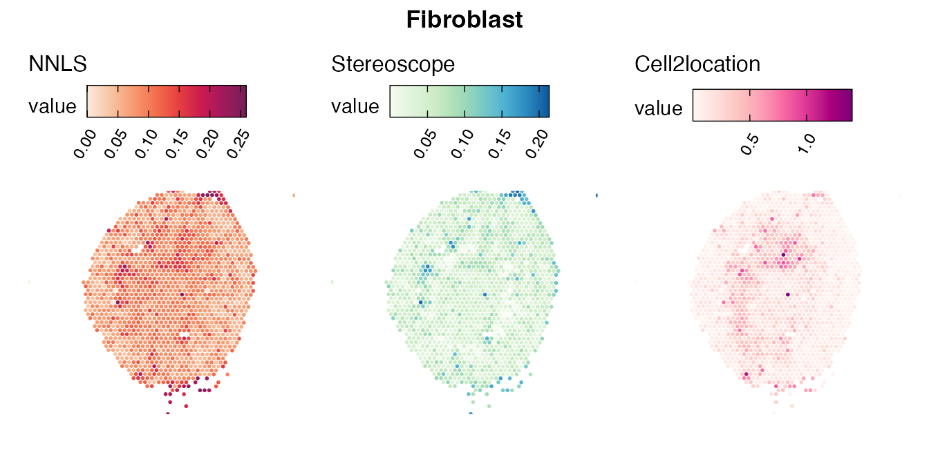
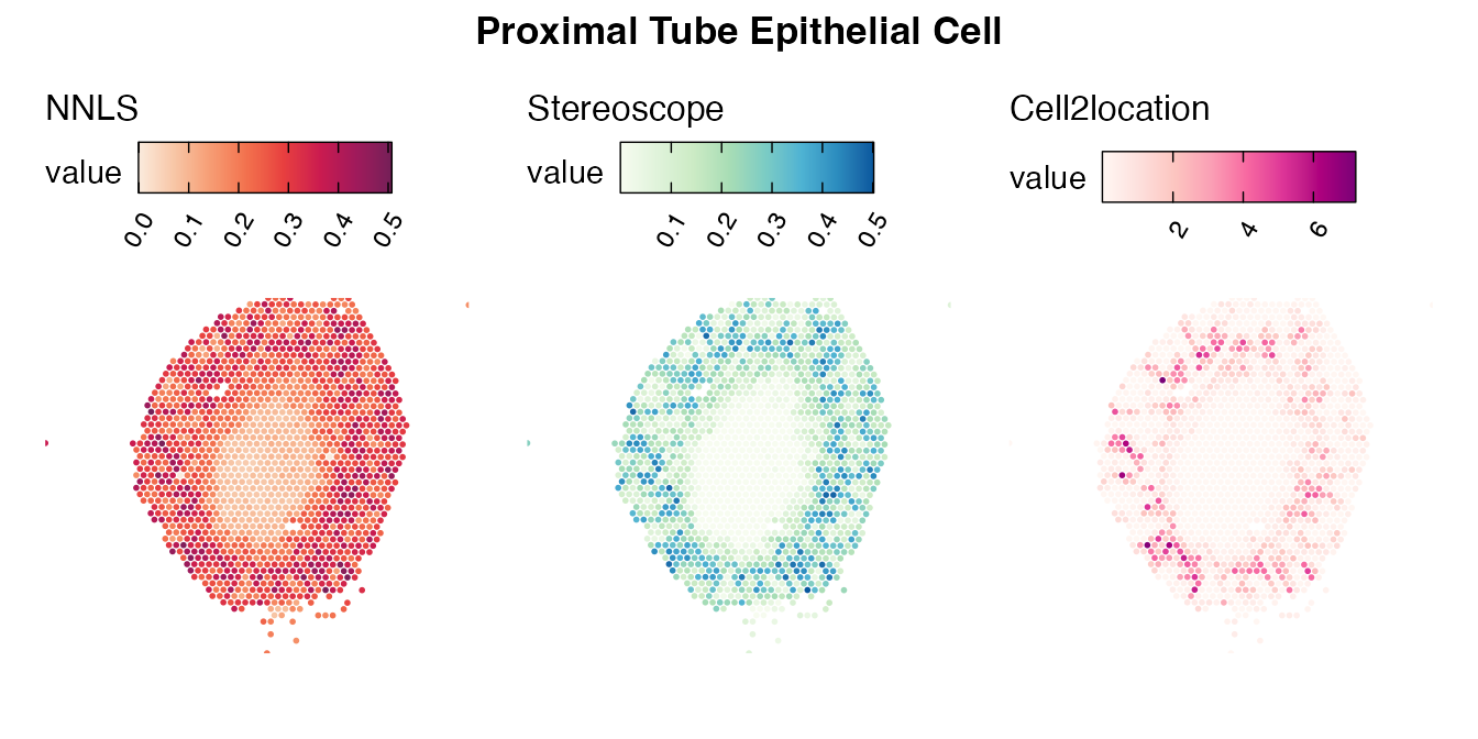
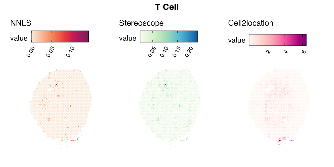
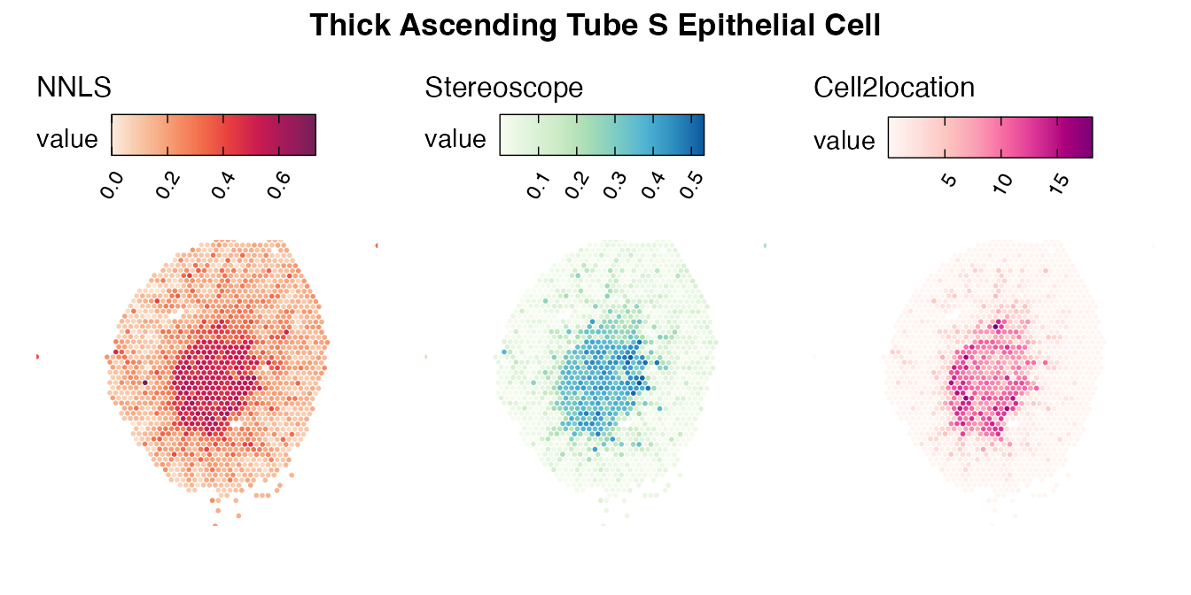
The same comparison approach as for the mouse brain data is applied to study the results for the mouse kidney sample, producing spot-wise correlation values between the cell type mapping results using the three different methods included for the comparison.
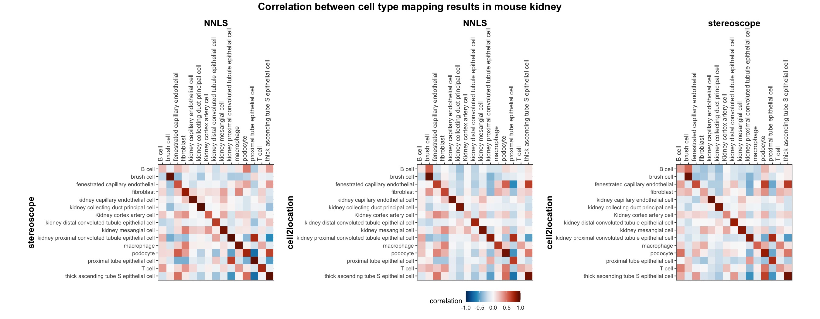
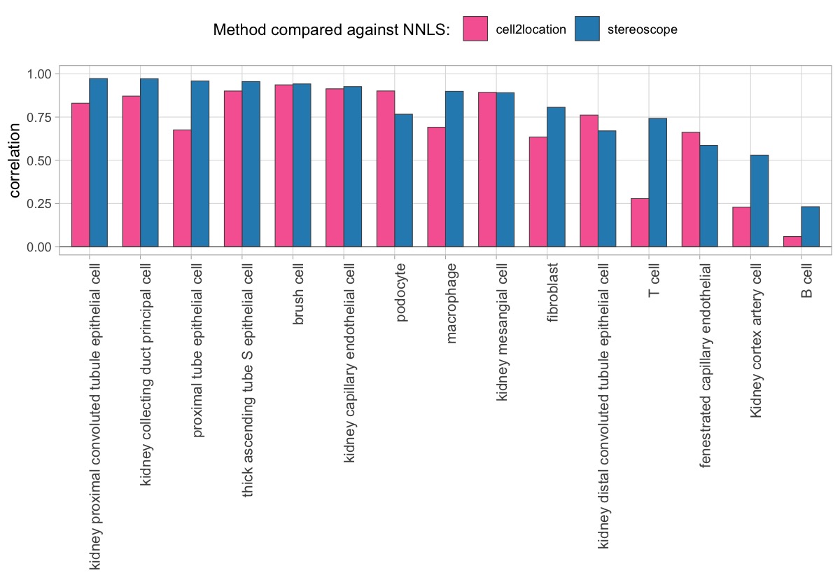
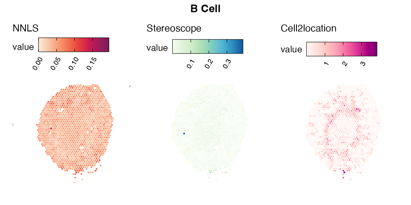
Also for this data set, there is an overall high cell-cell correlation between the NNLS results and those produced by stereoscope and cell2location. However, we can for instance see that all three methods seem to have difficulties correctly mapping B cells, as there seem to be very little concordance across the method mapping results.
Conclusion
In summary, we here demonstrate the utility of the NNLS approach for
cell type decomposition of Visium data, using two separate data sets, by
comparing it with two well established methods, stereoscope and
cell2location. Overall, the concordance in the inferred cell
type spot proportion is high between all methods, showing that NNLS is
an acceptable alternative for performing a fast cell type mapping
analysis of your Visium data, where a good reference scRNA-seq data set
is available. We would still recommend users to try out additional
methods on their data in order to fully appreciate the variability in
the mapping results that may occur due to design differences of these
algorithms. Nonetheless, the NNLS approach provided in
semla can act as an initial test ground for optimizing cell
type annotation levels or filtering parameters in a quick and versatile
fashion, before moving on to a slightly more computationally heavy
approach.
Package versions
-
semla: 1.4.1
Session info
## R version 4.4.2 (2024-10-31)
## Platform: aarch64-apple-darwin20.0.0
## Running under: macOS Sequoia 15.7.3
##
## Matrix products: default
## BLAS/LAPACK: /Users/javierescudero/miniconda3/envs/r-semlaupd/lib/libopenblas.0.dylib;  LAPACK version 3.12.0
##
## locale:
## [1] en_US.UTF-8/en_US.UTF-8/en_US.UTF-8/C/en_US.UTF-8/en_US.UTF-8
##
## time zone: Europe/Stockholm
## tzcode source: system (macOS)
##
## attached base packages:
## [1] stats     graphics  grDevices utils     datasets  methods   base
##
## other attached packages:
## [1] patchwork_1.3.1    tidyr_1.3.1        tibble_3.2.1       semla_1.4.1
## [5] ggplot2_3.5.2      dplyr_1.1.4        Seurat_5.3.0       SeuratObject_5.1.0
## [9] sp_2.2-0
##
## loaded via a namespace (and not attached):
##   [1] RColorBrewer_1.1-3     rstudioapi_0.17.1      jsonlite_1.9.0
##   [4] magrittr_2.0.3         spatstat.utils_3.1-4   magick_2.8.7
##   [7] farver_2.1.2           rmarkdown_2.29         fs_1.6.5
##  [10] ragg_1.3.3             vctrs_0.6.5            ROCR_1.0-11
##  [13] spatstat.explore_3.4-3 htmltools_0.5.8.1      forcats_1.0.0
##  [16] sass_0.4.9             sctransform_0.4.2      parallelly_1.42.0
##  [19] KernSmooth_2.23-26     bslib_0.9.0            htmlwidgets_1.6.4
##  [22] desc_1.4.3             ica_1.0-3              plyr_1.8.9
##  [25] plotly_4.11.0          zoo_1.8-13             cachem_1.1.0
##  [28] igraph_2.1.4           mime_0.12              lifecycle_1.0.4
##  [31] pkgconfig_2.0.3        Matrix_1.7-2           R6_2.6.1
##  [34] fastmap_1.2.0          fitdistrplus_1.2-3     future_1.34.0
##  [37] shiny_1.10.0           digest_0.6.37          colorspace_2.1-1
##  [40] tensor_1.5.1           RSpectra_0.16-2        irlba_2.3.5.1
##  [43] textshaping_0.4.0      labeling_0.4.3         progressr_0.15.1
##  [46] spatstat.sparse_3.1-0  httr_1.4.7             polyclip_1.10-7
##  [49] abind_1.4-5            compiler_4.4.2         withr_3.0.2
##  [52] viridis_0.6.5          fastDummies_1.7.5      MASS_7.3-64
##  [55] tools_4.4.2            lmtest_0.9-40          httpuv_1.6.15
##  [58] future.apply_1.11.3    goftest_1.2-3          glue_1.8.0
##  [61] dbscan_1.2.2           nlme_3.1-167           promises_1.3.2
##  [64] grid_4.4.2             Rtsne_0.17             cluster_2.1.8
##  [67] reshape2_1.4.4         generics_0.1.3         gtable_0.3.6
##  [70] spatstat.data_3.1-6    data.table_1.17.0      spatstat.geom_3.4-1
##  [73] RcppAnnoy_0.0.22       ggrepel_0.9.6          RANN_2.6.2
##  [76] pillar_1.10.1          stringr_1.5.1          spam_2.11-1
##  [79] RcppHNSW_0.6.0         later_1.4.1            splines_4.4.2
##  [82] lattice_0.22-6         survival_3.8-3         deldir_2.0-4
##  [85] tidyselect_1.2.1       miniUI_0.1.1.1         pbapply_1.7-2
##  [88] knitr_1.50             gridExtra_2.3          scattermore_1.2
##  [91] xfun_0.53              matrixStats_1.5.0      stringi_1.8.4
##  [94] lazyeval_0.2.2         yaml_2.3.10            evaluate_1.0.5
##  [97] codetools_0.2-20       cli_3.6.4              uwot_0.2.3
## [100] xtable_1.8-4           reticulate_1.42.0      systemfonts_1.3.1
## [103] munsell_0.5.1          jquerylib_0.1.4        Rcpp_1.1.0
## [106] globals_0.16.3         spatstat.random_3.4-1  zeallot_0.2.0
## [109] png_0.1-8              spatstat.univar_3.1-3  parallel_4.4.2
## [112] pkgdown_2.1.1          dotCall64_1.2          listenv_0.9.1
## [115] viridisLite_0.4.2      scales_1.3.0           ggridges_0.5.6
## [118] purrr_1.0.4            rlang_1.1.5            cowplot_1.1.3
## [121] shinyjs_2.1.0


