5.5 Non-negative matrix factorization

Another fun analysis to run is NMF, which is another dimensionality reduction method that has proven to be great at finding underlying patterns of transcriptomic profiles.

Briefly, starting with an expression matrix A with non-negative elements, NMF tries to decompose A into k preselected factors:

\[ A \approx W*H \]

A factor can be thought of as an expression profile that reflects some unknown signal of heterogeneity such as that of a cell type, multiple co-localized cell types or a biological process. From the resulting matrix H, we can extract information about the contribution of spots to each factor which allows us to visualize the factors on our tissue sections. From the second matrix W, we can extract information about the contribution of genes to each factor. In other words, we can both visualize the factors spatially and characterize them by their top contributing genes. Let’s have a look at an example:

se.cor <- RunNMF(se.cor, nfactors = 10)

In the plot below, we show five selected factors with their spatial distribution and top contributing genes.

FactorPlot <- function(object, 
                       factor = 1, 
                       col.scale = c("darkblue", "cyan", "yellow", "red", "darkred")
                       ) {
  p1 <- ST.DimPlot(object, 
                   dims = factor, 
                   label.by = "slide_id",
                   center.zero = F, 
                   reduction = "NMF", 
                   ncol = 2, 
                   pt.size = 1.3, 
                   cols = col.scale, 
                   show.sb = F) & labs(fill = "factor\nactivity")
  p2 <- FactorGeneLoadingPlot(object, 
                              factor = factor, 
                              dark.theme = F) + 
    labs(title = paste("Factor", factor, "loadings")) +
    theme(axis.title.y = element_blank()) & labs(y = "gene weight")
  cowplot::plot_grid(p1, p2, ncol = 2, rel_widths = c(2, 1))
}
# FactorPlot(object = se.cor, col.scale = col_scale)

plot_list <- lapply(1:10, function(i) {
  FactorPlot(object = se.cor, factor = i, col.scale = col_scale)
})

cowplot::plot_grid(plotlist = plot_list[c(1, 2, 4, 5, 9)], ncol = 1)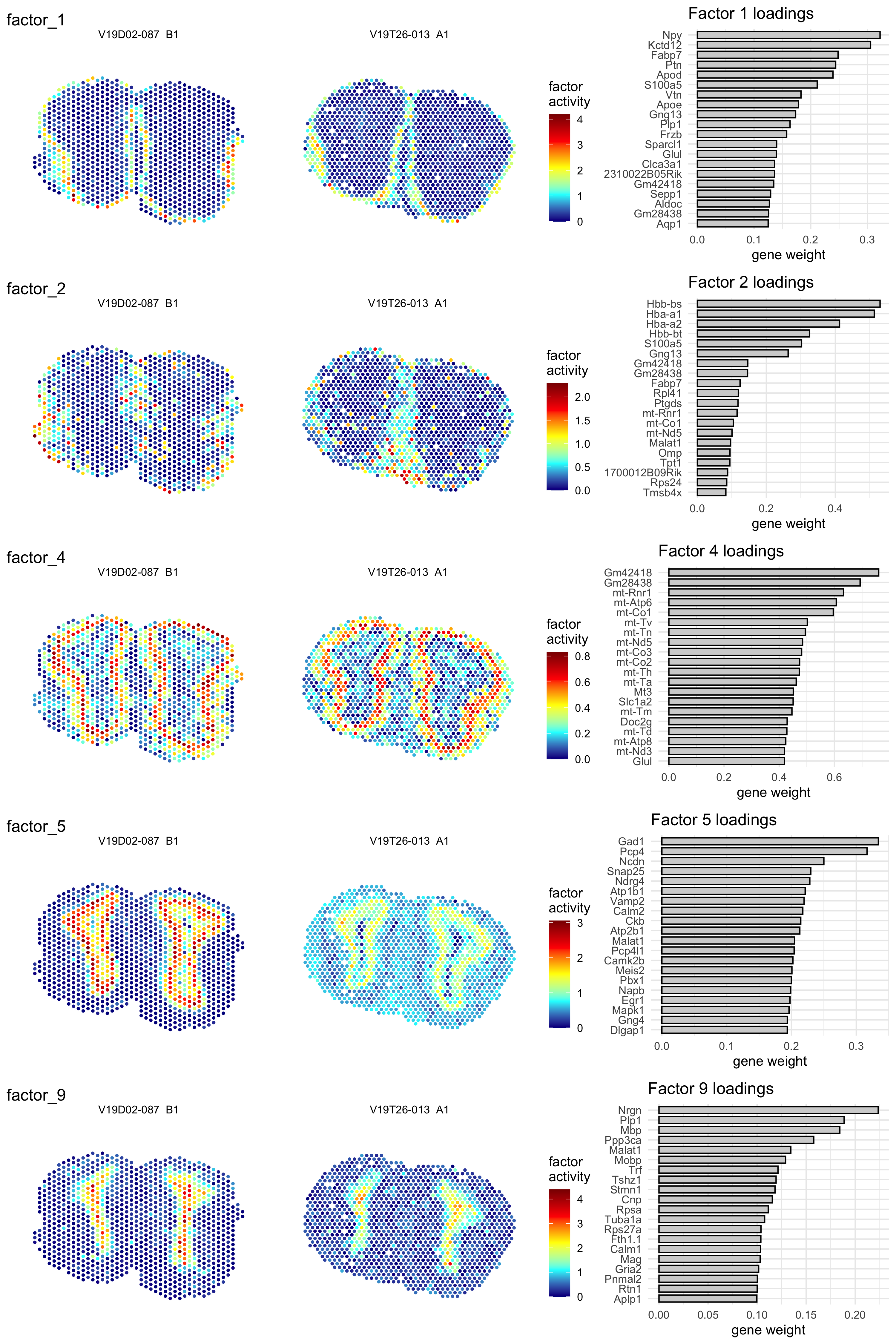

Figure 5.4: Five example factors from an NMF analysis with k = 10. The left hand side shows the activity of the factor on the tissue sections whereas the right hand side shows the top contributing genes with their associated weights

Looking at these results, you can see that some factors still display a large difference between the two sections, which is caused by the difference in quality. Even with an effective normalization procedure, some of the factor associated marker genes are still lowly expressed and/or have low detection rates. The NMF method does not operate on the integrated data and is therefore unable to adjust for strong batch effects. However, it is often possible to pick up signals of technical variation with NMF in which case such “technical” factors can be excluded.