4.1 Basic QC metrics

Plotting the spatial distribution of a certain QC metrics is often very useful. Below we show the distribution of unique genes and number of UMIs per spot in our two MOB tissue sections. By visual inspection we can see that both QC metrics correlate with cell density, which is what we generally expect to see. If this is not the case, we might have a technical issue such as tissue detachment, uneven permeabilization, overpermeabilization, mRNA degradation etc.

In this particular example, we see that even though the QC metrics correlate with cell density, there is a strong batch effect between the two sections where the second tissue section has much lower overall quality.

col_scale <- c("darkblue", "cyan", "yellow", "red", "darkred")
FeatureOverlay(se, features = c("nFeature_RNA", "nCount_RNA"), cols = col_scale, ncols = 2, 
               pt.size = 1.8, label.by = "slide_id", sampleids = 1:2, value.scale = "all")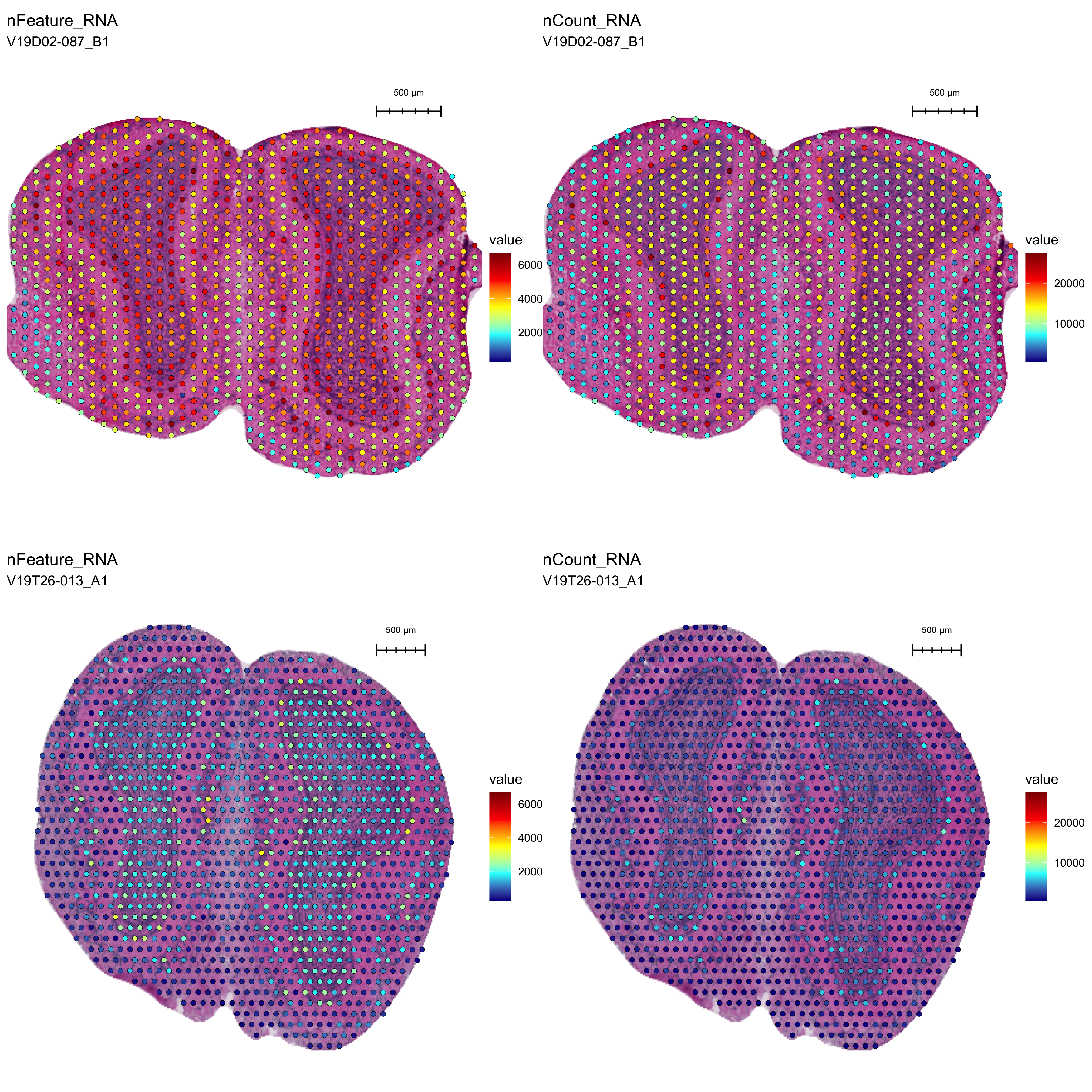

Figure 4.1: Spatial QC metrics overlay. nFeature_RNA = unique genes; nCount_RNA = UMI count

Visualizing the distribution of selected QC metrics can be useful to better understand the data. For example, if you need to select filtering thresholds.

For our example, it becomes clear that our two tissue section data sets are highly different in terms of quality. When analyzing a Visium data set generated from a new tissue type, it can be very difficult to determine whether the QC metrics are reasonable. Here, when comparing the two tissue sections side by side, it becomes clear that the second data set is of low quality. As a rule of thumb, we expect to obtain at least 1,000 unique genes per spot on average but you should know that this is highly tissue dependent. Low quality will have a negative impact on downstream analysis.

col_samples <- c("#1954A6", "#A7C947")
p1 <- ggplot() +
  geom_histogram(data = se[[]], aes(nFeature_RNA, fill = slide_id), alpha = 0.6, bins = 50, position = "identity") +
  scale_fill_manual(values = col_samples) +
  ggtitle("A) Unique genes per spot") & NoLegend()

p2 <- ggplot() +
  geom_histogram(data = se[[]], aes(nCount_RNA, fill = slide_id), alpha = 0.6, bins = 50, position = "identity") +
  scale_fill_manual(values = col_samples) +
  ggtitle("B) Total counts per spot") & NoLegend()

gene_attr <- rbind(data.frame(nUMI = Matrix::rowSums(se@assays$RNA@counts[, se$slide_id == "V19D02-087_B1"]), 
                        nSpots = Matrix::rowSums(se@assays$RNA@counts[, se$slide_id == "V19D02-087_B1"] > 0),
                        slide_id = "V19D02-087_B1"),
                   data.frame(nUMI = Matrix::rowSums(se@assays$RNA@counts[, se$slide_id == "V19T26-013_A1"]), 
                        nSpots = Matrix::rowSums(se@assays$RNA@counts[, se$slide_id == "V19T26-013_A1"] > 0),
                        slide_id = "V19T26-013_A1"))
p3 <- ggplot() +
  geom_histogram(data = gene_attr, aes(nUMI, fill = slide_id), alpha = 0.6, bins = 50, position = "identity") +
  scale_fill_manual(values = col_samples) +
  scale_x_log10() +
  ggtitle("C) Total counts per gene (log10 scale)")

p4 <- ggplot() +
  geom_histogram(data = gene_attr, aes(nSpots, fill = slide_id), alpha = 0.6,  bins = 50, position = "identity") +
  scale_fill_manual(values = col_samples) +
  ggtitle("D) Total spots per gene")

(p1 - p2)/(p3 - p4) & theme_linedraw()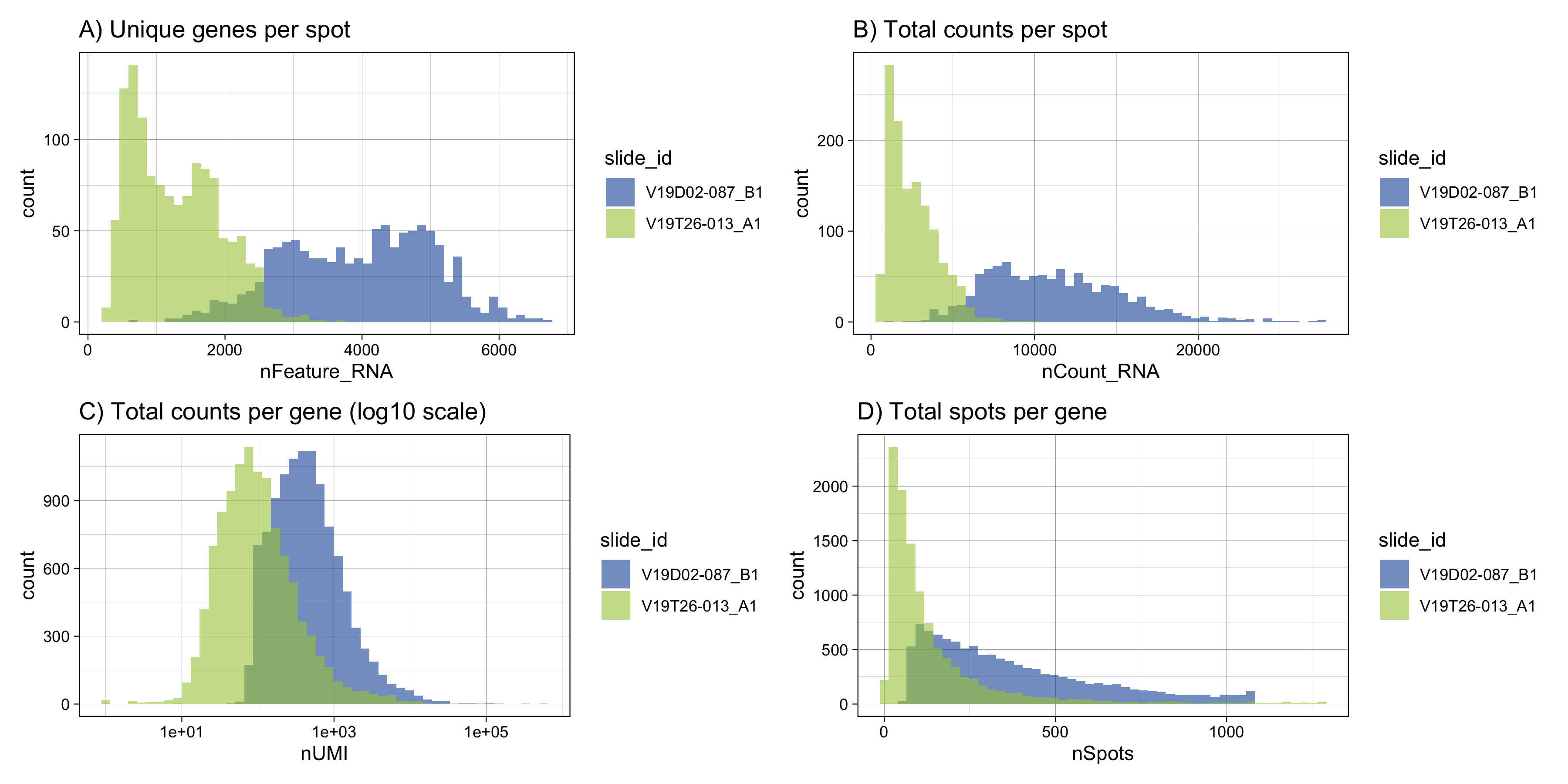

Figure 4.2: Visualization of basic QC metrics. A) Histogram of unique genes per spot. B) Histogram of total UMI counts per spot. C) Total counts per gene in log10-scale. This is useful to inspect if you need to filter out lowly expressed genes from your data set. D) Total spots per gene. Here we can clearly see a substantial gene dropout in the low quality data set.