5.6 Clustering

We can use the harmonized PC vectors (integrated) as input for the clustering algorithm.

se.cor <- FindNeighbors(object = se.cor, verbose = T, reduction = "harmony", dims = 1:20)
se.cor <- FindClusters(se.cor)

col_clusters <- RColorBrewer::brewer.pal(9, name = "Set3")
p1 <- ST.FeaturePlot(se.cor, features = "seurat_clusters", ncol = 2, cols = col_clusters, label.by = "slide_id", show.sb = FALSE, pt.size = 1.5) + labs(title = "Clusters") & NoLegend()
p2 <- DimPlot(se.cor, reduction = "umap.harmony", group.by = "seurat_clusters", cols = col_clusters) + labs(title="UMAP")

p1 - p2 + patchwork::plot_layout(widths = c(3, 2))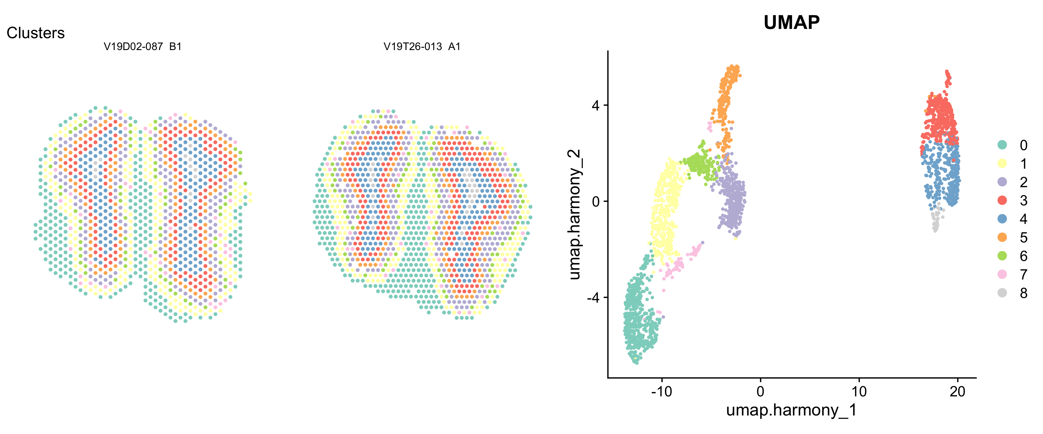

It looks like the clusters corresponds pretty well with the different layers in the MOB tissue. If we’d like, we can make some annotations for these clusters and correlate them to the anatomical layers.

cluster_annotations <- c(
  "L09", #0
  "L08", #1 
  "L05", #2
  "L03", #3
  "L02", #4
  "L04", #5
  "L06", #6
  "L07", #7
  "L01"  #8
  )
se.cor$cluster_annotation <- factor(plyr::mapvalues(x = Idents(se.cor), from = 0:8, to = cluster_annotations), 
                                              levels = c(paste0("L0", 1:9)))

col_spectral <- RColorBrewer::brewer.pal(9, name = "Spectral")
# p1 <- ST.FeaturePlot(se.cor, features = "cluster_annotation", ncol = 2, cols = col_spectral) + labs(title="Clusters") & NoLegend()
# p2 <- DimPlot(se.cor, reduction = "umap.harmony", group.by = "cluster_annotation", cols = col_spectral) + labs(title="UMAP")

ST.FeaturePlot(se.cor, features = "cluster_annotation", ncol = 2, cols = col_spectral, show.sb = F, dark.theme = T, pt.size = 2, label.by = "slide_id") + labs(title="")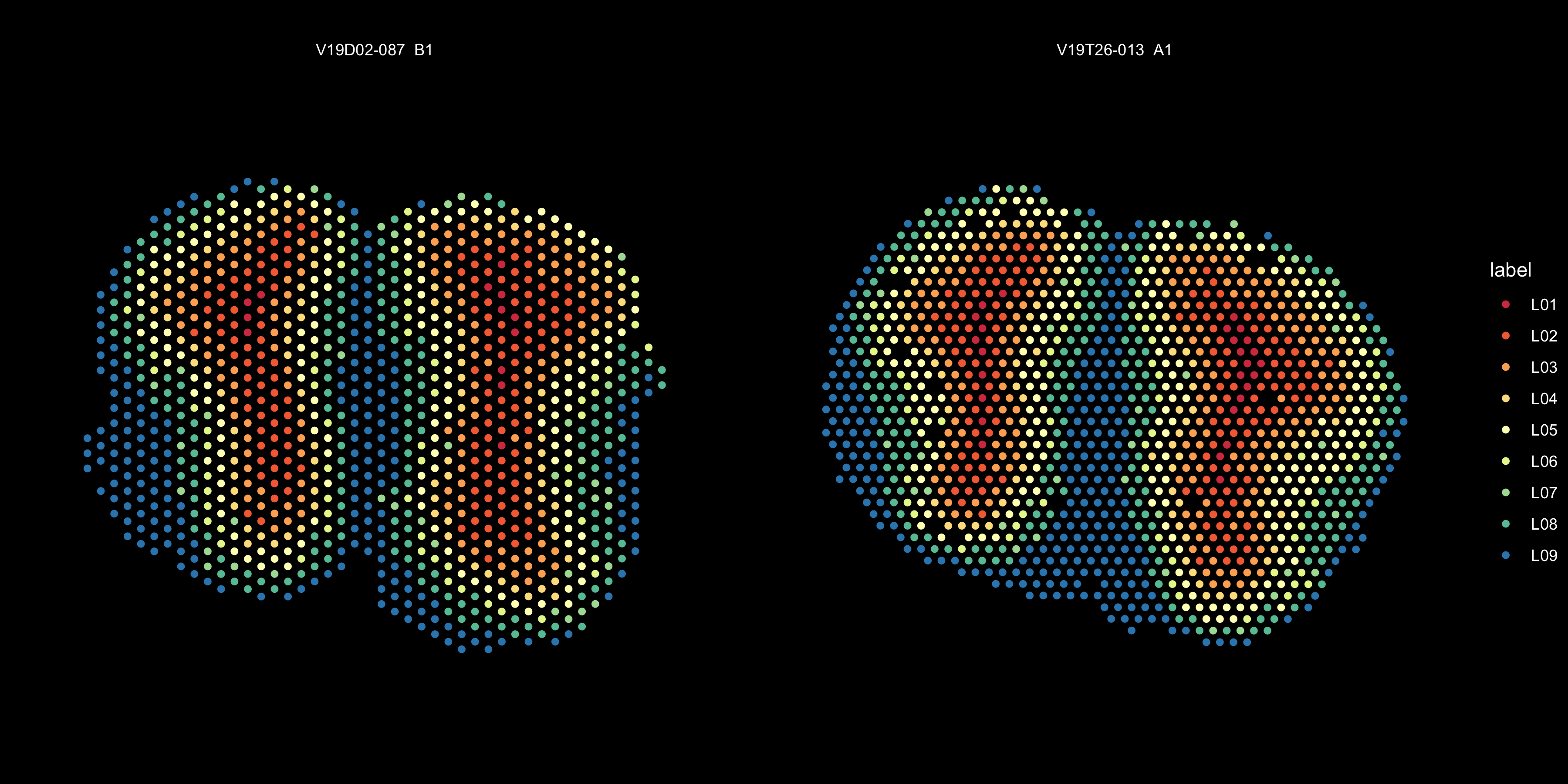

Figure 5.5: Spatial distribution of clusters

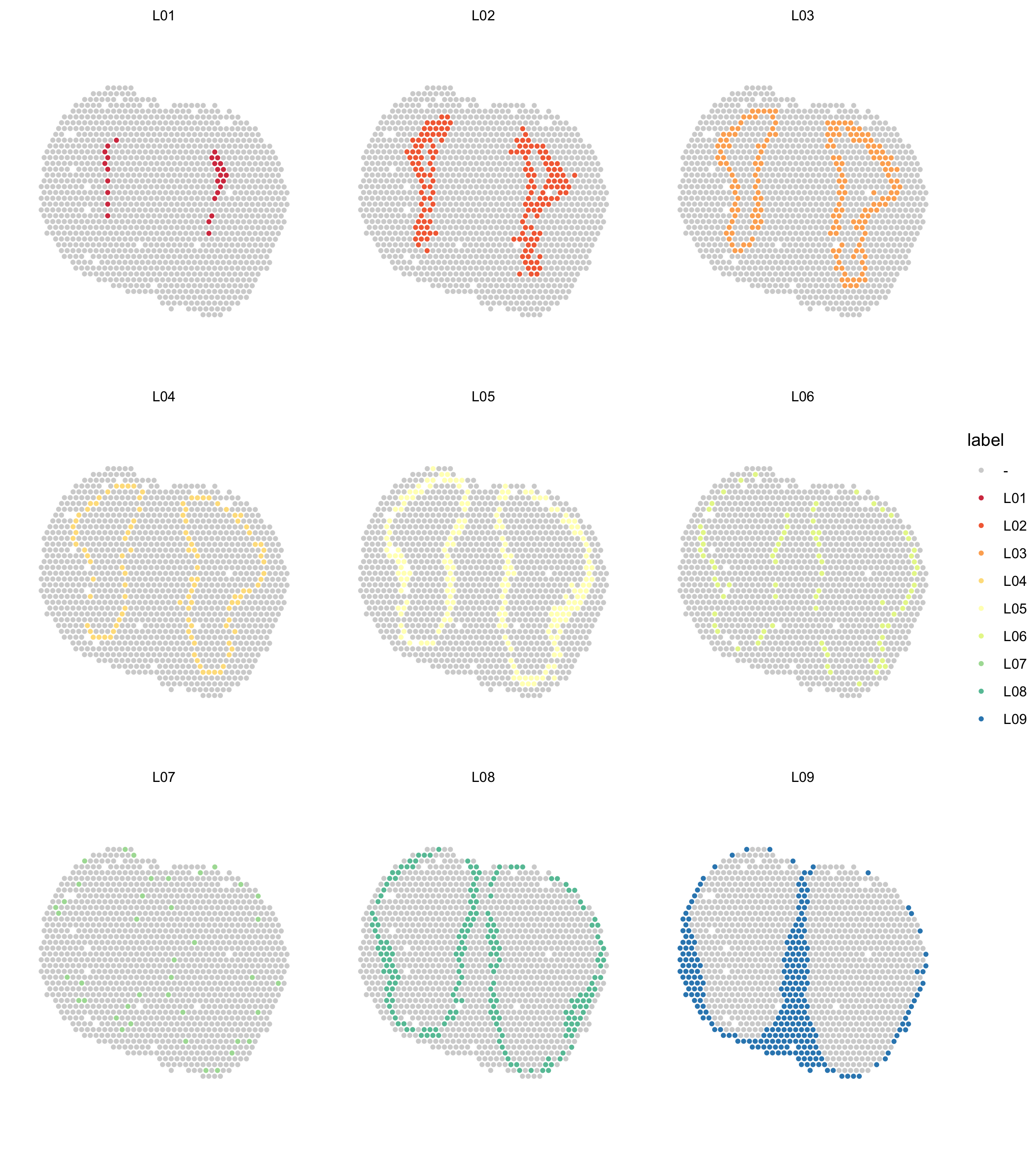
We can also plot the clusters one by one;

col_spectral <- RColorBrewer::brewer.pal(9, name = "Spectral")
ST.FeaturePlot(se.cor, 
               features = "cluster_annotation", 
               indices = 2, 
               cols = col_spectral,
               split.labels = T, 
               pt.size = 1.5, 
               ncol = 3, 
               show.sb = F) & 
  theme(plot.title = element_blank())