Subset/merge
Last updated: 2022-02-28
Checks: 7 0
Knit directory: STUtility_web_site/
This reproducible R Markdown analysis was created with workflowr (version 1.7.0). The Checks tab describes the reproducibility checks that were applied when the results were created. The Past versions tab lists the development history.
Great! Since the R Markdown file has been committed to the Git repository, you know the exact version of the code that produced these results.
Great job! The global environment was empty. Objects defined in the global environment can affect the analysis in your R Markdown file in unknown ways. For reproduciblity it’s best to always run the code in an empty environment.
The command set.seed(20191031) was run prior to running the code in the R Markdown file. Setting a seed ensures that any results that rely on randomness, e.g. subsampling or permutations, are reproducible.
Great job! Recording the operating system, R version, and package versions is critical for reproducibility.
Nice! There were no cached chunks for this analysis, so you can be confident that you successfully produced the results during this run.
Great job! Using relative paths to the files within your workflowr project makes it easier to run your code on other machines.
Great! You are using Git for version control. Tracking code development and connecting the code version to the results is critical for reproducibility.
The results in this page were generated with repository version 64ae8be. See the Past versions tab to see a history of the changes made to the R Markdown and HTML files.
Note that you need to be careful to ensure that all relevant files for the analysis have been committed to Git prior to generating the results (you can use wflow_publish or wflow_git_commit). workflowr only checks the R Markdown file, but you know if there are other scripts or data files that it depends on. Below is the status of the Git repository when the results were generated:
Ignored files:
    Ignored:    .Rhistory
    Ignored:    analysis/.DS_Store
    Ignored:    analysis/manual_annotation.png
    Ignored:    pre_data/
Note that any generated files, e.g. HTML, png, CSS, etc., are not included in this status report because it is ok for generated content to have uncommitted changes.
These are the previous versions of the repository in which changes were made to the R Markdown (analysis/Subset_and_Merge.Rmd) and HTML (docs/Subset_and_Merge.html) files. If you’ve configured a remote Git repository (see ?wflow_git_remote), click on the hyperlinks in the table below to view the files as they were in that past version.
| File | Version | Author | Date | Message |
|---|---|---|---|---|
| html | d41bcb0 | Ludvig Larsson | 2022-02-28 | Build site. |
| html | 0dafcee | Ludvig Larsson | 2021-05-06 | Build site. |
| Rmd | b7a0414 | Ludvig Larsson | 2021-05-06 | Updated tutorials |
Subsetting
A Seurat object created with the STutility workflow contain special S4 class object called Staffli. In order to use STutility fucntions for plotting and image processing, this object needs to be present as it holds all the data related to the HE images and spatial coordinates. Unfortunately, this means that the generic functions typically used for subsetting and merging; subset and merge, will not work as expected. Instead, you should use the SubsetSTData and MergeSTData functions to perform the two operations.
For example, let’s say that we want to subset our Seurat object to include spots with at least 2000 unique genes. For this we can use SubsetSTData. Under the hood, SubsetSTData calls the generic function subset (see ?subset.Seurat for details), but in addition it will make sure that the Staffli object is also subsetted properly.
se.subset <- SubsetSTData(se, expression = nFeature_RNA >= 2000)
cat("Number of spots before filtering:", ncol(se), "\n")
Number of spots before filtering: 5053 cat("Number of spots after filtering:", ncol(se.subset), "\n")Number of spots after filtering: 4937 The expression argument allows you to evaluate any feature/variable pulled by FetchData so you can for example use this argument to subset based on meta.data columns or genes. You can also just specify the spot IDs that you want to keep to subset the data.
se.subset <- SubsetSTData(se, spots = colnames(se)[1:2000])
cat("Number of spots before filtering:", ncol(se), "\n")
Number of spots before filtering: 5053 cat("Number of spots after filtering:", ncol(se.subset), "\n")Number of spots after filtering: 2000 p1 <- ST.FeaturePlot(se, features = "nFeature_RNA")
p2 <- ST.FeaturePlot(se.subset, features = "nFeature_RNA", pt.size = 2)
p1 - p2 + patchwork::plot_layout(widths = c(1, 2))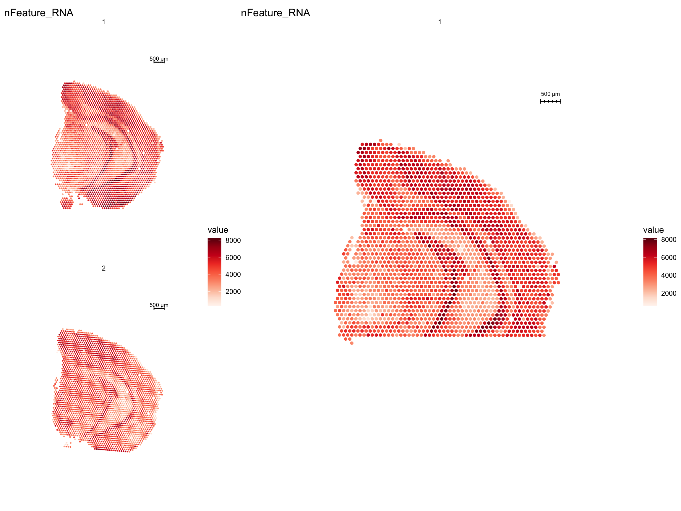
| Version | Author | Date |
|---|---|---|
| 0dafcee | Ludvig Larsson | 2021-05-06 |
Alternatively, if you want to filter the object at the gene level, you can use the features argument.
se.subset <- SubsetSTData(se, features = VariableFeatures(se))
cat("Number of genes before filtering:", nrow(se), "\n")
Number of genes before filtering: 13437 cat("Number of genes after filtering:", nrow(se.subset), "\n")Number of genes after filtering: 3000 If you want to subset one or several specific section(s) you just need a group variable in your meta.data slot. If you don’t have one it’s really easy to create one by pulling out the “sample” column from the Staffli object meta.data slot.
se$sample_id <- paste0("section_", GetStaffli(se)@meta.data$sample)

# Select section 2
se.subset <- SubsetSTData(se, expression = sample_id %in% "section_2")
cat("Number of spots before filtering:", ncol(se), "\n")
Number of spots before filtering: 5053 cat("Number of spots after filtering:", ncol(se.subset), "\n")Number of spots after filtering: 2496 p1 <- ST.FeaturePlot(se, features = "nFeature_RNA")
p2 <- ST.FeaturePlot(se.subset, features = "nFeature_RNA", pt.size = 2)
p1 - p2 + patchwork::plot_layout(widths = c(1, 2))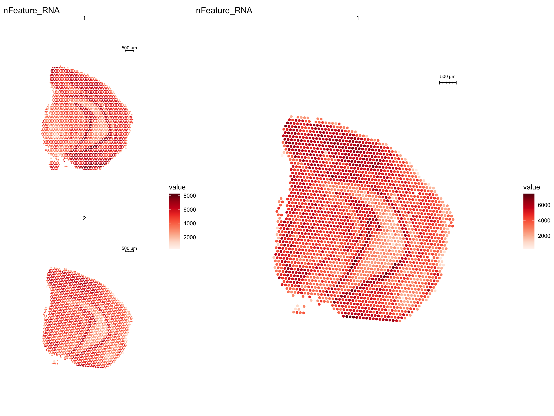
| Version | Author | Date |
|---|---|---|
| 0dafcee | Ludvig Larsson | 2021-05-06 |
Merging
If you want to merge data, you will have to use the MergeSTData function to make sure that the Staffli objects are merged properly. Same as for the SubsetSTData, MergeSTData calls the generic function merge (see ?merge.Seurat) under the hood and then merges the Staffli objects.
# Create subsets
se1 <- SubsetSTData(se, expression = sample_id %in% "section_1")
se2 <- SubsetSTData(se, expression = sample_id %in% "section_2")

se.merged <- MergeSTData(se1, se2)

ST.FeaturePlot(se.merged, features = "nFeature_RNA", ncol = 2)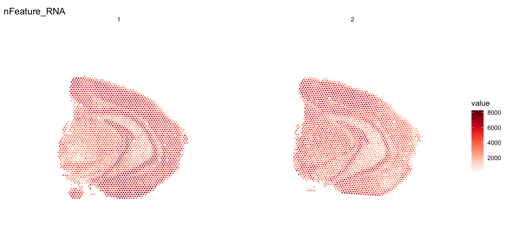
| Version | Author | Date |
|---|---|---|
| 0dafcee | Ludvig Larsson | 2021-05-06 |
You can also merge multiple samples at the same time if you put the second argument as a list of Seurat objects.
se.merged <- MergeSTData(se1, y = list(se2, se3, se4))A work by Joseph Bergenstråhle and Ludvig Larsson
sessionInfo()R version 4.0.3 (2020-10-10)
Platform: x86_64-apple-darwin13.4.0 (64-bit)
Running under: macOS Mojave 10.14.6
Matrix products: default
BLAS/LAPACK: /Users/ludviglarsson/anaconda3/envs/R4.0/lib/libopenblasp-r0.3.12.dylib
locale:
[1] en_US.UTF-8/en_US.UTF-8/en_US.UTF-8/C/en_US.UTF-8/en_US.UTF-8
attached base packages:
[1] stats graphics grDevices utils datasets methods base
other attached packages:
[1] magrittr_2.0.1 kableExtra_1.3.4 STutility_0.1.0 ggplot2_3.3.5
[5] SeuratObject_4.0.0 Seurat_4.0.2 workflowr_1.7.0
loaded via a namespace (and not attached):
[1] utf8_1.2.1 reticulate_1.18 tidyselect_1.1.1
[4] htmlwidgets_1.5.3 grid_4.0.3 Rtsne_0.15
[7] munsell_0.5.0 codetools_0.2-18 ica_1.0-2
[10] units_0.7-1 future_1.21.0 miniUI_0.1.1.1
[13] withr_2.4.1 colorspace_2.0-0 highr_0.8
[16] knitr_1.31 uuid_0.1-4 rstudioapi_0.13
[19] ROCR_1.0-11 tensor_1.5 listenv_0.8.0
[22] labeling_0.4.2 git2r_0.28.0 polyclip_1.10-0
[25] farver_2.1.0 rprojroot_2.0.2 coda_0.19-4
[28] parallelly_1.25.0 LearnBayes_2.15.1 vctrs_0.3.8
[31] generics_0.1.0 xfun_0.20 R6_2.5.0
[34] doParallel_1.0.16 Morpho_2.8 ggiraph_0.7.8
[37] manipulateWidget_0.11.0 spatstat.utils_2.2-0 assertthat_0.2.1
[40] promises_1.2.0.1 scales_1.1.1 imager_0.42.8
[43] gtable_0.3.0 globals_0.14.0 bmp_0.3
[46] processx_3.5.1 goftest_1.2-2 rlang_1.0.1
[49] zeallot_0.1.0 akima_0.6-2.1 systemfonts_1.0.1
[52] splines_4.0.3 lazyeval_0.2.2 spatstat.geom_2.3-0
[55] rgl_0.105.22 yaml_2.2.1 reshape2_1.4.4
[58] abind_1.4-5 crosstalk_1.1.1 httpuv_1.5.5
[61] tools_4.0.3 spData_0.3.8 ellipsis_0.3.2
[64] spatstat.core_2.3-0 raster_3.4-10 jquerylib_0.1.3
[67] RColorBrewer_1.1-2 proxy_0.4-25 Rvcg_0.19.2
[70] ggridges_0.5.3 Rcpp_1.0.6 plyr_1.8.6
[73] classInt_0.4-3 purrr_0.3.4 ps_1.6.0
[76] rpart_4.1-15 dbscan_1.1-6 deldir_1.0-6
[79] pbapply_1.4-3 viridis_0.6.1 cowplot_1.1.1
[82] zoo_1.8-9 ggrepel_0.9.1 cluster_2.1.1
[85] colorRamps_2.3 fs_1.5.0 data.table_1.14.0
[88] magick_2.7.2 scattermore_0.7 readbitmap_0.1.5
[91] gmodels_2.18.1 lmtest_0.9-38 RANN_2.6.1
[94] whisker_0.4 fitdistrplus_1.1-3 matrixStats_0.58.0
[97] patchwork_1.1.1 shinyjs_2.0.0 mime_0.10
[100] evaluate_0.14 xtable_1.8-4 jpeg_0.1-8.1
[103] gridExtra_2.3 compiler_4.0.3 tibble_3.1.6
[106] KernSmooth_2.23-18 crayon_1.4.1 htmltools_0.5.1.1
[109] mgcv_1.8-34 later_1.1.0.1 spdep_1.1-7
[112] tiff_0.1-8 tidyr_1.2.0 expm_0.999-6
[115] DBI_1.1.1 MASS_7.3-53.1 sf_0.9-8
[118] boot_1.3-27 Matrix_1.3-2 cli_3.1.1
[121] gdata_2.18.0 parallel_4.0.3 igraph_1.2.6
[124] pkgconfig_2.0.3 getPass_0.2-2 sp_1.4-5
[127] plotly_4.9.3 spatstat.sparse_2.0-0 xml2_1.3.2
[130] foreach_1.5.1 svglite_2.0.0 bslib_0.2.4
[133] webshot_0.5.2 rvest_1.0.0 stringr_1.4.0
[136] callr_3.7.0 digest_0.6.27 sctransform_0.3.2
[139] RcppAnnoy_0.0.18 spatstat.data_2.1-0 rmarkdown_2.7
[142] leiden_0.3.7 uwot_0.1.10 gdtools_0.2.3
[145] shiny_1.6.0 gtools_3.8.2 lifecycle_1.0.1
[148] nlme_3.1-152 jsonlite_1.7.2 viridisLite_0.4.0
[151] fansi_0.4.2 pillar_1.7.0 lattice_0.20-41
[154] fastmap_1.1.0 httr_1.4.2 survival_3.2-10
[157] glue_1.4.2 png_0.1-7 iterators_1.0.13
[160] class_7.3-18 stringi_1.5.3 sass_0.3.1
[163] dplyr_1.0.8 irlba_2.3.3 e1071_1.7-6
[166] future.apply_1.7.0