3D visualization
Last updated: 2022-02-28
Checks: 7 0
Knit directory: STUtility_web_site/
This reproducible R Markdown analysis was created with workflowr (version 1.7.0). The Checks tab describes the reproducibility checks that were applied when the results were created. The Past versions tab lists the development history.
Great! Since the R Markdown file has been committed to the Git repository, you know the exact version of the code that produced these results.
Great job! The global environment was empty. Objects defined in the global environment can affect the analysis in your R Markdown file in unknown ways. For reproduciblity it’s best to always run the code in an empty environment.
The command set.seed(20191031) was run prior to running the code in the R Markdown file. Setting a seed ensures that any results that rely on randomness, e.g. subsampling or permutations, are reproducible.
Great job! Recording the operating system, R version, and package versions is critical for reproducibility.
Nice! There were no cached chunks for this analysis, so you can be confident that you successfully produced the results during this run.
Great job! Using relative paths to the files within your workflowr project makes it easier to run your code on other machines.
Great! You are using Git for version control. Tracking code development and connecting the code version to the results is critical for reproducibility.
The results in this page were generated with repository version 64ae8be. See the Past versions tab to see a history of the changes made to the R Markdown and HTML files.
Note that you need to be careful to ensure that all relevant files for the analysis have been committed to Git prior to generating the results (you can use wflow_publish or wflow_git_commit). workflowr only checks the R Markdown file, but you know if there are other scripts or data files that it depends on. Below is the status of the Git repository when the results were generated:
Ignored files:
Ignored: .Rhistory
Ignored: analysis/.DS_Store
Ignored: analysis/manual_annotation.png
Ignored: pre_data/
Note that any generated files, e.g. HTML, png, CSS, etc., are not included in this status report because it is ok for generated content to have uncommitted changes.
These are the previous versions of the repository in which changes were made to the R Markdown (analysis/3D_visualization.Rmd) and HTML (docs/3D_visualization.html) files. If you’ve configured a remote Git repository (see ?wflow_git_remote), click on the hyperlinks in the table below to view the files as they were in that past version.
| File | Version | Author | Date | Message |
|---|---|---|---|---|
| html | d41bcb0 | Ludvig Larsson | 2022-02-28 | Build site. |
| html | bb6466f | Ludvig Larsson | 2022-02-28 | Build site. |
| Rmd | 060b185 | Ludvig Larsson | 2021-06-29 | Added link to README |
| html | 0dafcee | Ludvig Larsson | 2021-05-06 | Build site. |
| html | df62517 | Ludvig Larsson | 2021-05-06 | Build site. |
| html | 88b046f | Ludvig Larsson | 2021-05-05 | Build site. |
| html | f34bd02 | Ludvig Larsson | 2021-05-05 | wflow_git_commit(all = TRUE) |
| Rmd | f8f90b4 | Ludvig Larsson | 2021-05-05 | wflow_git_commit(all = TRUE) |
| html | e0390c8 | Ludvig Larsson | 2021-05-05 | Update |
| html | 4af6496 | Ludvig Larsson | 2021-05-05 | Updated tutorials |
| html | b88bd19 | Ludvig Larsson | 2021-05-05 | Build site. |
| html | e526be2 | Ludvig Larsson | 2021-05-05 | Build site. |
| html | 3a8eb02 | Ludvig Larsson | 2021-05-04 | Build site. |
| Rmd | dfc9b23 | Ludvig Larsson | 2021-05-04 | Added split data tutorial |
| html | 395091f | Ludvig Larsson | 2021-05-04 | Build site. |
| html | da131a6 | Ludvig Larsson | 2021-05-04 | Build site. |
| html | 3ef1b70 | Ludvig Larsson | 2021-05-04 | Build site. |
| html | 9fe84d9 | Ludvig Larsson | 2021-05-04 | Build site. |
| html | bfe87d1 | Ludvig Larsson | 2021-05-04 | Build site. |
| Rmd | eba61ce | Ludvig Larsson | 2021-05-04 | Updated website with new theme and content |
| html | 1dc000c | Ludvig Larsson | 2021-04-28 | Build site. |
| html | 1e9c615 | Ludvig Larsson | 2021-04-28 | Build site. |
| Rmd | 83100ed | Ludvig Larsson | 2021-04-28 | wflow_publish(files = c("analysis/index.Rmd", "analysis/about.Rmd", |
| html | 34884bd | Ludvig Larsson | 2020-10-06 | Build site. |
| html | d13dabd | Ludvig Larsson | 2020-06-05 | Build site. |
| html | 60407bb | Ludvig Larsson | 2020-06-05 | Build site. |
| html | e339ebc | Ludvig Larsson | 2020-06-05 | Build site. |
| Rmd | 42cb54d | Ludvig Larsson | 2020-06-05 | downsampled points in 3D visualization |
| html | 6606127 | Ludvig Larsson | 2020-06-05 | Build site. |
| html | f0ea9c1 | Ludvig Larsson | 2020-06-05 | Build site. |
| html | 651f315 | Ludvig Larsson | 2020-06-05 | Build site. |
| Rmd | 98f1fe2 | Ludvig Larsson | 2020-06-05 | downsampled points in 3D visualization |
| html | a6a0c51 | Ludvig Larsson | 2020-06-05 | Build site. |
| html | f3c5cb4 | Ludvig Larsson | 2020-06-05 | Build site. |
| html | f89df7e | Ludvig Larsson | 2020-06-05 | Build site. |
| Rmd | 672b4e5 | Ludvig Larsson | 2020-06-05 | downsampled points in 3D visualization |
| html | 1e67a7c | Ludvig Larsson | 2020-06-04 | Build site. |
| html | f71b0c0 | Ludvig Larsson | 2020-06-04 | Build site. |
| html | 4c48cfa | Ludvig Larsson | 2020-06-04 | Build site. |
| Rmd | a0ea32a | Ludvig Larsson | 2020-06-04 | update website |
| html | 23df05c | jbergenstrahle | 2020-01-11 | Build site. |
| Rmd | efbbda3 | jbergenstrahle | 2020-01-01 | update pek |
| Rmd | 672191f | Ludvig Larsson | 2019-12-16 | Added 3D plotting to vignette |
| html | 672191f | Ludvig Larsson | 2019-12-16 | Added 3D plotting to vignette |
Creating 3D stack of points
STutility currently allows for visualization of features in 3D using a point cloud created from the nuclei detected in aligned HE images using the Create3DStack() function. The cell nuclei coordinates are extracted based on color intensity as nuclei are typically darker in color than the surrounding tissue. This is not an exact cell segmentation but it will typically capture the density of nuclei well enough to define various morphological structures.
Once the nuclei coordinates have been extracted from each aligned section, a z value will be assigned to each section to create a 3D stack. Feature values can be interpolated across the points in the stack and then visualized in 3D by mapping the values to a colorscale. Below are a couple of criteria that has to be fulfilled for the method to work:
- The sections have to come from the same tissue type with similar morphology for each section
- HE image has to be aligned, i.e. you have to run
LoadImages(),MaskImages()andAlignImages()(orManualAlignImages()) first - The images have to be loaded in higher resolution than the default 400 pixels. The
Create3DStack()will automatically reload the images in higher resolution if the image widths are lower than 400 pixels or you can runSwitchResolution()to reload the images in higher resolution before runningCreate3DStack() - The cell segmentation is based on color intensity and might therefore fail if artifacts are present in the HE images. This could for example be classifications, hair, folds, bubbles or dust. Uneven section thickness and staining can also affect the segmentation performance.
- It is assumed that the tissue sections have been stained with Hematoxylin and Eosin
Once the stack has been created, a 2D grid will be created that covers the aligned tissue sections with its width determined by the nx parameter. This grid will later be used to interpolate feature values over, so that we can assign a value to each point in the point cloud.
se <- Create3DStack(se)Point patterns
We can plot the stacked coordinates in 2D to see what the point patterns look like. From the plot below you can see that a higher density of points is picked up in areas width darker color, which is typically the case for the tissue edges.
stack_3d <- setNames(GetStaffli(se)@scatter.data, c("x", "y", "z", "grid.cell"))
ggplot(stack_3d, aes(x, 2e3 - y)) +
geom_point(size = 0.1, color = "lightgray") +
facet_wrap(~z, ncol = 1) +
theme_void()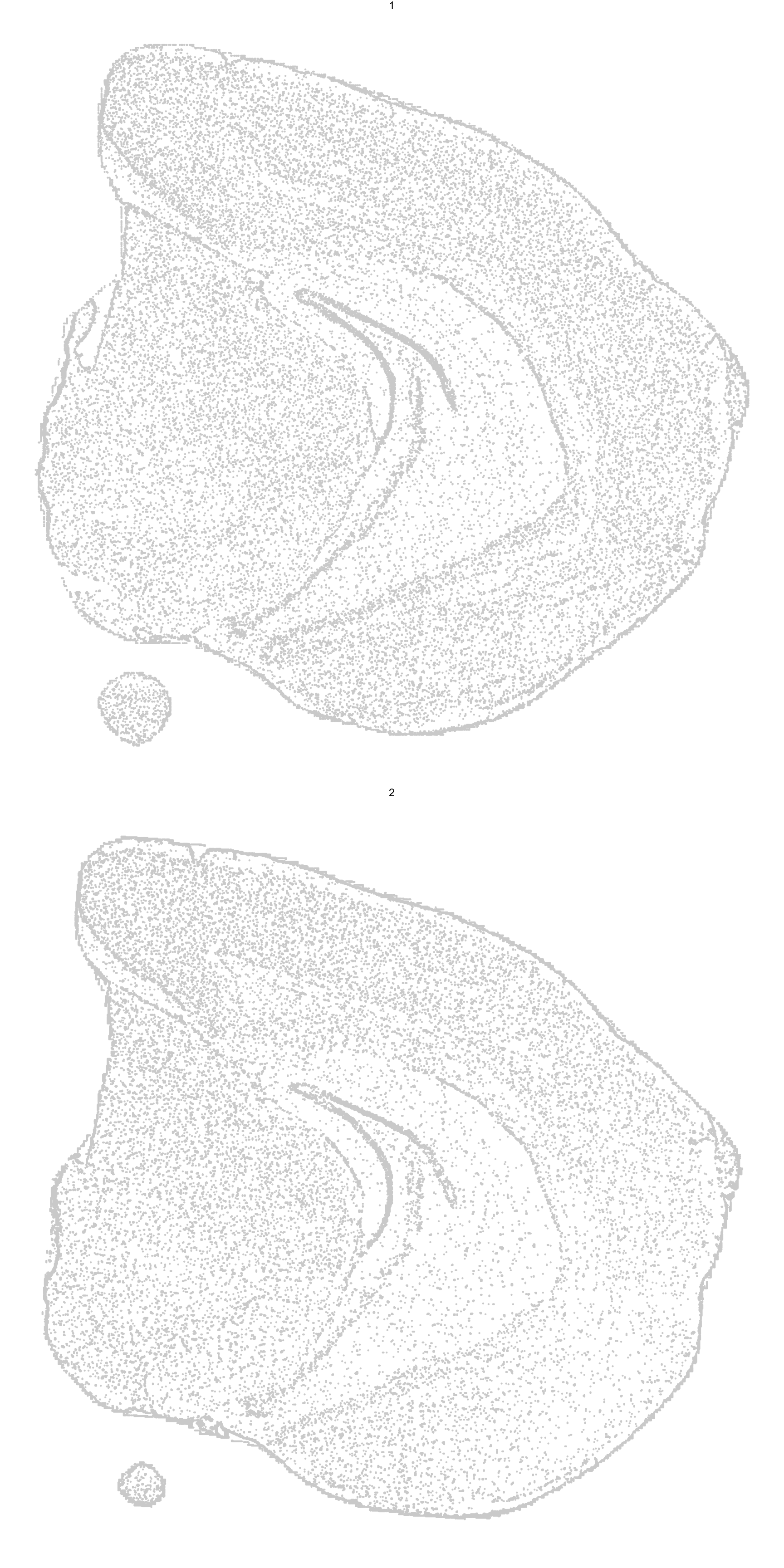
Data interpolation
The next step to visualize features is to interpolate values across the point patterns. Since each point is assigned to a grid cell, we can interpolate values across the grid and assign an interpolated values back to the points. Remember that the width of the grid is determined by the nx parameter and you can increase the resolution of the interpolation by setting nx to a higher value when running the Create3DStack() function. Increasing the value of this parameter will improve the “smoothness” of the colormap but will slow down the computation significantly.
interpolated.data <- FeaturePlot3D(se, features = "Mbp", return.data = TRUE)
ggplot(interpolated.data, aes(x, 2e3 - y, color = val)) +
geom_point(size = 0.1) +
facet_wrap(~z, ncol = 1) +
theme_void() +
ggtitle("Mbp") +
scale_color_gradientn(colours = c("black", "dark blue", "cyan", "yellow", "red", "dark red"))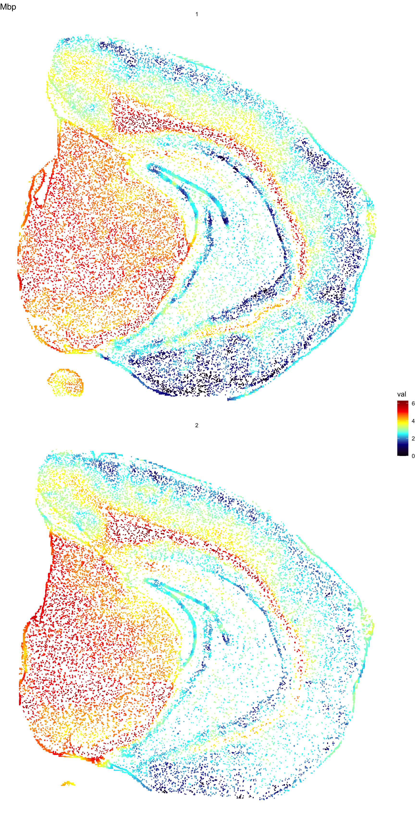
3D plot
To generate 3D plots you can use the visualization functions FeaturePlot3D(), DimPlot3D(), and HSVPlot3D(). Each section will by default be assigned a z coordinate ranging from 1 to N where N is the number of samples. If you wish to change these z coordinates you can use the parameter zcoords to map each section to a new value (note that you need to provide as many z coordinates as the number of samples in your Seurat object).
If you wish to force the sections closer to each other you can add margins to the z axis using the add.margins parameter. This will essentially add empty space below and above the 3D stack and therefore push the sections closer.
Now we are ready to plot features in 3D. We’ll run the FeaturePlot3D() function as above but with return.data = FALSE.
FeaturePlot3D(se, features = "Mbp", pt.size = 0.6, pts.downsample = 5e4)jpeg(filename = "~/Downloads/HippoHE.jpg", width = 3000, height = 1600, res = 300)
ImagePlot(se, method="raster", annotate = F)
dev.off()quartz_off_screen
2 Various other features and analysis results can be visualized, e.g. if we previously had performed a factor analysis on the samples, we can for example show theses factors simultaneously using the HSV color coding scheme. Just keep in mind that the factors needs to be non-overlapping. The HSV color scheme can be useful to show mulltiple features simultaneously, but it’s recommended to also explore the features one by one.
selected.factors <- paste0("factor_", c(4, 5, 7, 9, 11, 13, 14, 15, 18, 22, 24, 25, 29, 30, 31, 33, 36))
HSVPlot3D(se, features = selected.factors, pt.size = 2, add.margins = 1, mode = "spots")Multiple 3D plots
The 3D plots are drawn using the plotly R package and you can specify a layout attribute called scene to the FeaturePlot3D() to enable the visualization of multiple 3D plots at the same time. Below we plot the features “Mbp” and “Calb2” in two different scenes and we can then use subplot() to visualize them side by side.
p1 <- FeaturePlot3D(se, features = "Mbp", scene = "scene", cols = c("dark blue", "navyblue", "cyan", "white"), add.margins = 1, pts.downsample = 5e4)
p2 <- FeaturePlot3D(se, features = "Calb2", scene = "scene2", cols = c("dark blue", "navyblue", "cyan", "white"), add.margins = 1)
plotly::subplot(p1, p2, margin = 0)A work by Joseph Bergenstråhle and Ludvig Larsson
sessionInfo()R version 4.0.3 (2020-10-10)
Platform: x86_64-apple-darwin13.4.0 (64-bit)
Running under: macOS Mojave 10.14.6
Matrix products: default
BLAS/LAPACK: /Users/ludviglarsson/anaconda3/envs/R4.0/lib/libopenblasp-r0.3.12.dylib
locale:
[1] en_US.UTF-8/en_US.UTF-8/en_US.UTF-8/C/en_US.UTF-8/en_US.UTF-8
attached base packages:
[1] stats graphics grDevices utils datasets methods base
other attached packages:
[1] STutility_0.1.0 ggplot2_3.3.5 SeuratObject_4.0.0 Seurat_4.0.2
[5] workflowr_1.7.0
loaded via a namespace (and not attached):
[1] utf8_1.2.1 reticulate_1.18 tidyselect_1.1.1
[4] htmlwidgets_1.5.3 grid_4.0.3 Rtsne_0.15
[7] munsell_0.5.0 codetools_0.2-18 ica_1.0-2
[10] units_0.7-1 future_1.21.0 miniUI_0.1.1.1
[13] withr_2.4.1 colorspace_2.0-0 highr_0.8
[16] knitr_1.31 uuid_0.1-4 rstudioapi_0.13
[19] ROCR_1.0-11 tensor_1.5 listenv_0.8.0
[22] labeling_0.4.2 git2r_0.28.0 polyclip_1.10-0
[25] farver_2.1.0 rprojroot_2.0.2 coda_0.19-4
[28] parallelly_1.25.0 LearnBayes_2.15.1 vctrs_0.3.8
[31] generics_0.1.0 xfun_0.20 R6_2.5.0
[34] doParallel_1.0.16 Morpho_2.8 ggiraph_0.7.8
[37] manipulateWidget_0.11.0 spatstat.utils_2.2-0 assertthat_0.2.1
[40] promises_1.2.0.1 scales_1.1.1 imager_0.42.8
[43] gtable_0.3.0 globals_0.14.0 bmp_0.3
[46] processx_3.5.1 goftest_1.2-2 rlang_1.0.1
[49] zeallot_0.1.0 akima_0.6-2.1 systemfonts_1.0.1
[52] splines_4.0.3 lazyeval_0.2.2 spatstat.geom_2.3-0
[55] rgl_0.105.22 yaml_2.2.1 reshape2_1.4.4
[58] abind_1.4-5 crosstalk_1.1.1 httpuv_1.5.5
[61] tools_4.0.3 spData_0.3.8 ellipsis_0.3.2
[64] spatstat.core_2.3-0 raster_3.4-10 jquerylib_0.1.3
[67] RColorBrewer_1.1-2 proxy_0.4-25 Rvcg_0.19.2
[70] ggridges_0.5.3 Rcpp_1.0.6 plyr_1.8.6
[73] classInt_0.4-3 purrr_0.3.4 ps_1.6.0
[76] rpart_4.1-15 dbscan_1.1-6 deldir_1.0-6
[79] pbapply_1.4-3 viridis_0.6.1 cowplot_1.1.1
[82] zoo_1.8-9 ggrepel_0.9.1 cluster_2.1.1
[85] colorRamps_2.3 fs_1.5.0 magrittr_2.0.1
[88] data.table_1.14.0 magick_2.7.2 scattermore_0.7
[91] readbitmap_0.1.5 gmodels_2.18.1 lmtest_0.9-38
[94] RANN_2.6.1 whisker_0.4 fitdistrplus_1.1-3
[97] matrixStats_0.58.0 patchwork_1.1.1 shinyjs_2.0.0
[100] mime_0.10 evaluate_0.14 xtable_1.8-4
[103] jpeg_0.1-8.1 gridExtra_2.3 compiler_4.0.3
[106] tibble_3.1.6 KernSmooth_2.23-18 crayon_1.4.1
[109] htmltools_0.5.1.1 mgcv_1.8-34 later_1.1.0.1
[112] spdep_1.1-7 tiff_0.1-8 tidyr_1.2.0
[115] expm_0.999-6 DBI_1.1.1 MASS_7.3-53.1
[118] sf_0.9-8 boot_1.3-27 Matrix_1.3-2
[121] cli_3.1.1 gdata_2.18.0 parallel_4.0.3
[124] igraph_1.2.6 pkgconfig_2.0.3 getPass_0.2-2
[127] sp_1.4-5 plotly_4.9.3 spatstat.sparse_2.0-0
[130] foreach_1.5.1 bslib_0.2.4 stringr_1.4.0
[133] callr_3.7.0 digest_0.6.27 sctransform_0.3.2
[136] RcppAnnoy_0.0.18 spatstat.data_2.1-0 rmarkdown_2.7
[139] leiden_0.3.7 uwot_0.1.10 gdtools_0.2.3
[142] shiny_1.6.0 gtools_3.8.2 lifecycle_1.0.1
[145] nlme_3.1-152 jsonlite_1.7.2 viridisLite_0.4.0
[148] fansi_0.4.2 pillar_1.7.0 lattice_0.20-41
[151] fastmap_1.1.0 httr_1.4.2 survival_3.2-10
[154] glue_1.4.2 png_0.1-7 iterators_1.0.13
[157] class_7.3-18 stringi_1.5.3 sass_0.3.1
[160] dplyr_1.0.8 irlba_2.3.3 e1071_1.7-6
[163] future.apply_1.7.0