Maize embryonic leaf analysis and z-stack
Last updated: 2022-02-28
Checks: 7 0
Knit directory: STUtility_web_site/
This reproducible R Markdown analysis was created with workflowr (version 1.7.0). The Checks tab describes the reproducibility checks that were applied when the results were created. The Past versions tab lists the development history.
Great! Since the R Markdown file has been committed to the Git repository, you know the exact version of the code that produced these results.
Great job! The global environment was empty. Objects defined in the global environment can affect the analysis in your R Markdown file in unknown ways. For reproduciblity it’s best to always run the code in an empty environment.
The command set.seed(20191031) was run prior to running the code in the R Markdown file. Setting a seed ensures that any results that rely on randomness, e.g. subsampling or permutations, are reproducible.
Great job! Recording the operating system, R version, and package versions is critical for reproducibility.
Nice! There were no cached chunks for this analysis, so you can be confident that you successfully produced the results during this run.
Great job! Using relative paths to the files within your workflowr project makes it easier to run your code on other machines.
Great! You are using Git for version control. Tracking code development and connecting the code version to the results is critical for reproducibility.
The results in this page were generated with repository version 64ae8be. See the Past versions tab to see a history of the changes made to the R Markdown and HTML files.
Note that you need to be careful to ensure that all relevant files for the analysis have been committed to Git prior to generating the results (you can use wflow_publish or wflow_git_commit). workflowr only checks the R Markdown file, but you know if there are other scripts or data files that it depends on. Below is the status of the Git repository when the results were generated:
Ignored files:
    Ignored:    .Rhistory
    Ignored:    analysis/.DS_Store
    Ignored:    analysis/manual_annotation.png
    Ignored:    pre_data/
Note that any generated files, e.g. HTML, png, CSS, etc., are not included in this status report because it is ok for generated content to have uncommitted changes.
These are the previous versions of the repository in which changes were made to the R Markdown (analysis/Maize_data.Rmd) and HTML (docs/Maize_data.html) files. If you’ve configured a remote Git repository (see ?wflow_git_remote), click on the hyperlinks in the table below to view the files as they were in that past version.
| File | Version | Author | Date | Message |
|---|---|---|---|---|
| Rmd | 64ae8be | Ludvig Larsson | 2022-02-28 | Updated tutorials |
| html | d41bcb0 | Ludvig Larsson | 2022-02-28 | Build site. |
| html | ea27662 | Ludvig Larsson | 2022-02-28 | Build site. |
| Rmd | 1d8db06 | Ludvig Larsson | 2022-02-28 | Incldued new walkthrough |
| html | 1d8db06 | Ludvig Larsson | 2022-02-28 | Incldued new walkthrough |
| Rmd | a13f35b | Ludvig Larsson | 2022-02-28 | Added walkthrough |
library(Seurat)
library(magrittr)
library(imager)
library(EBImage)
library(STutility)
library(magrittr)
library(dplyr)
library(harmony)
samples <- "data/filtered_feature_bc_matrix.h5"
imgs <- "data/tissue_hires_image.png"
spotfiles <- "data/tissue_positions_list.csv"
json <- "data/scalefactors_json.json"
infoTable <- data.frame(samples, imgs, spotfiles, json)
se <- InputFromTable(infoTable)Manual selection
Here we manually annotated the four section as “group1” - “group4”.
se <- LoadImages(se, time.resolve = FALSE)
se <- ManualAnnotation(se)
First, let’s have a look at the histological image and then overlay our selections on top of it.
ImagePlot(se, method = "raster", annotate = FALSE)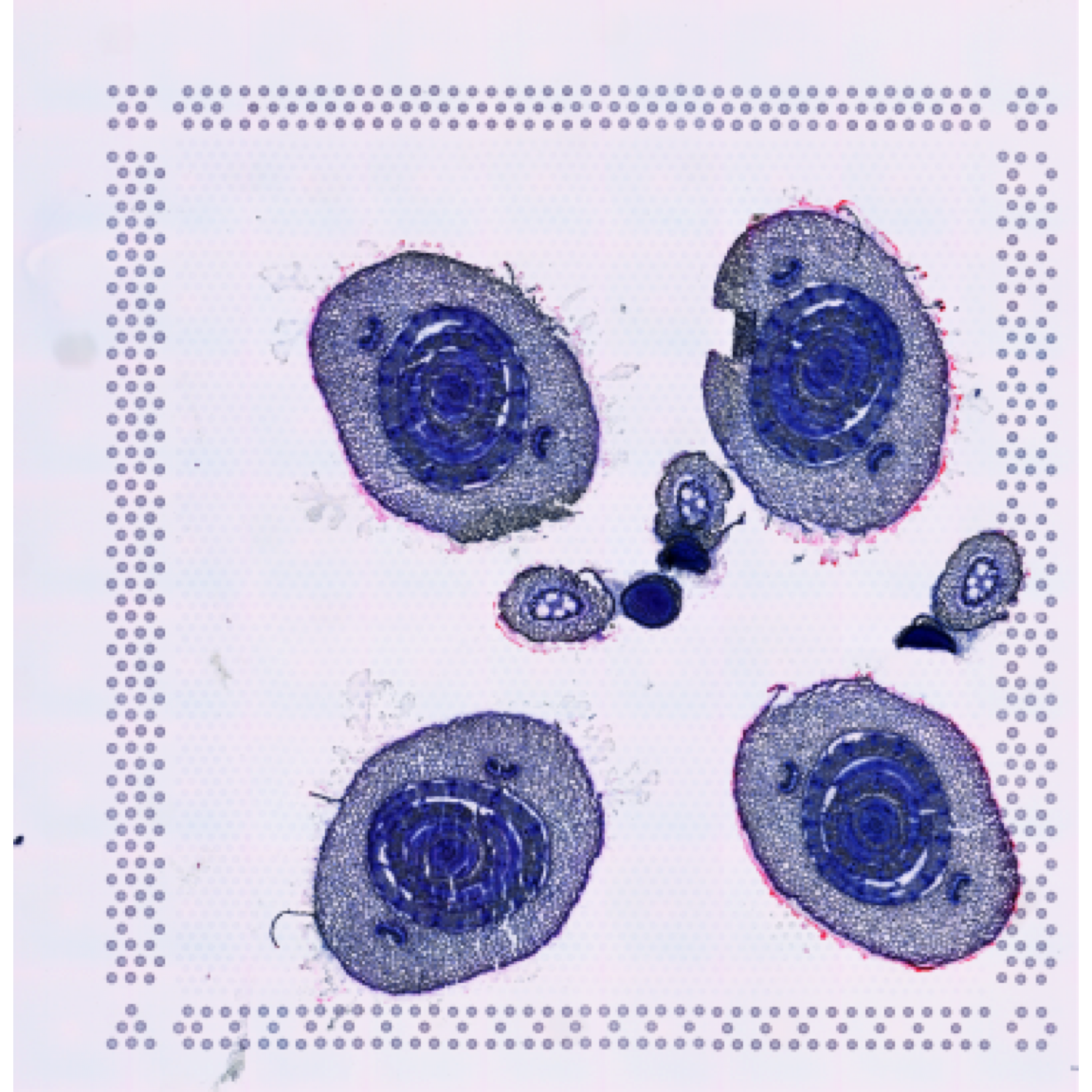
| Version | Author | Date |
|---|---|---|
| 1d8db06 | Ludvig Larsson | 2022-02-28 |
FeatureOverlay(se, features = "labels")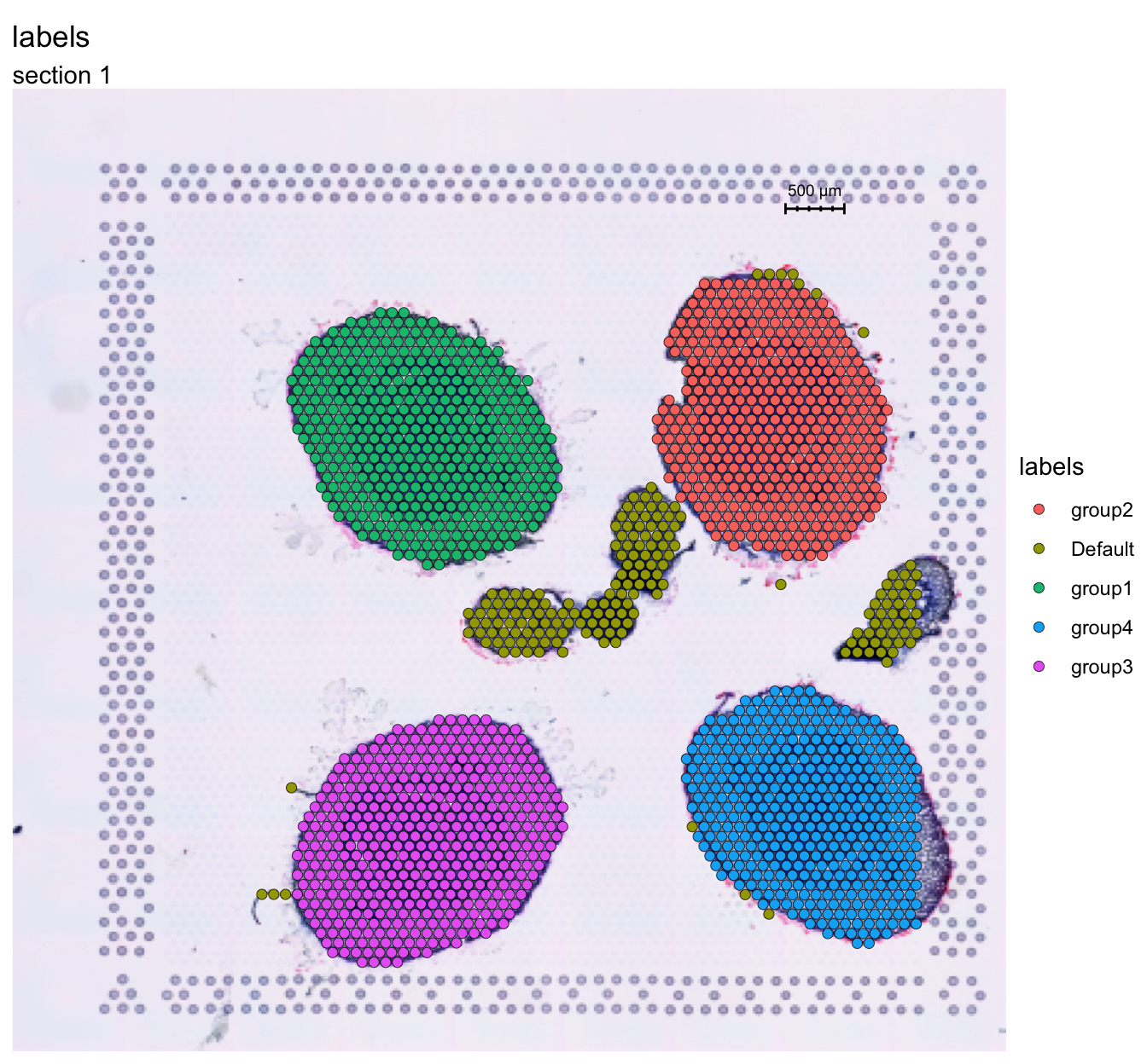
| Version | Author | Date |
|---|---|---|
| 1d8db06 | Ludvig Larsson | 2022-02-28 |
Find “crop windows”
We can use the GetCropWindows function to extract “crop geometries” which we will be using to crop the data. Since we have four tissue sections in diofferent orientation, it is more convenient to work with the data if we can split each section into a separate dataset.
crop.geoms <- GetCropWindows(se, groups.to.keep = paste0("group", 1:4))
crop.geoms
$`1`
geom group group.by
"620x623+499+416" "group1" "labels"
$`1`
geom group group.by
"551x664+1216+356" "group2" "labels"
$`1`
geom group group.by
"621x603+509+1262" "group3" "labels"
$`1`
geom group group.by
"551x623+1273+1202" "group4" "labels" The ´crop.geoms´ is a list where each element is named by section id (for example “1” above since all crop windows come from section 1) and contain a vector with: (1) a string which defines the width, height and offset along the x and y axes, (2) the group column name and (3) the group variable name. The latter two are required to make sure that spots are only selected from the correct group regardless if the cropped images overlap with another group.
To illustrate this, we can plot the “crop windows” on our histological image:
im <- magick::image_read(GetStaffli(se)@imgs[1]) %>% imager::magick2cimg()corners <- apply(do.call(rbind, sapply(crop.geoms, function(x) {
strsplit(x[1], "x|\\+")
})), 2, as.numeric)
plot(im)
rect(xleft = corners[, 3], ybottom = corners[, 4], xright = corners[, 3] + corners[, 1], ytop = corners[, 4] + corners[, 2])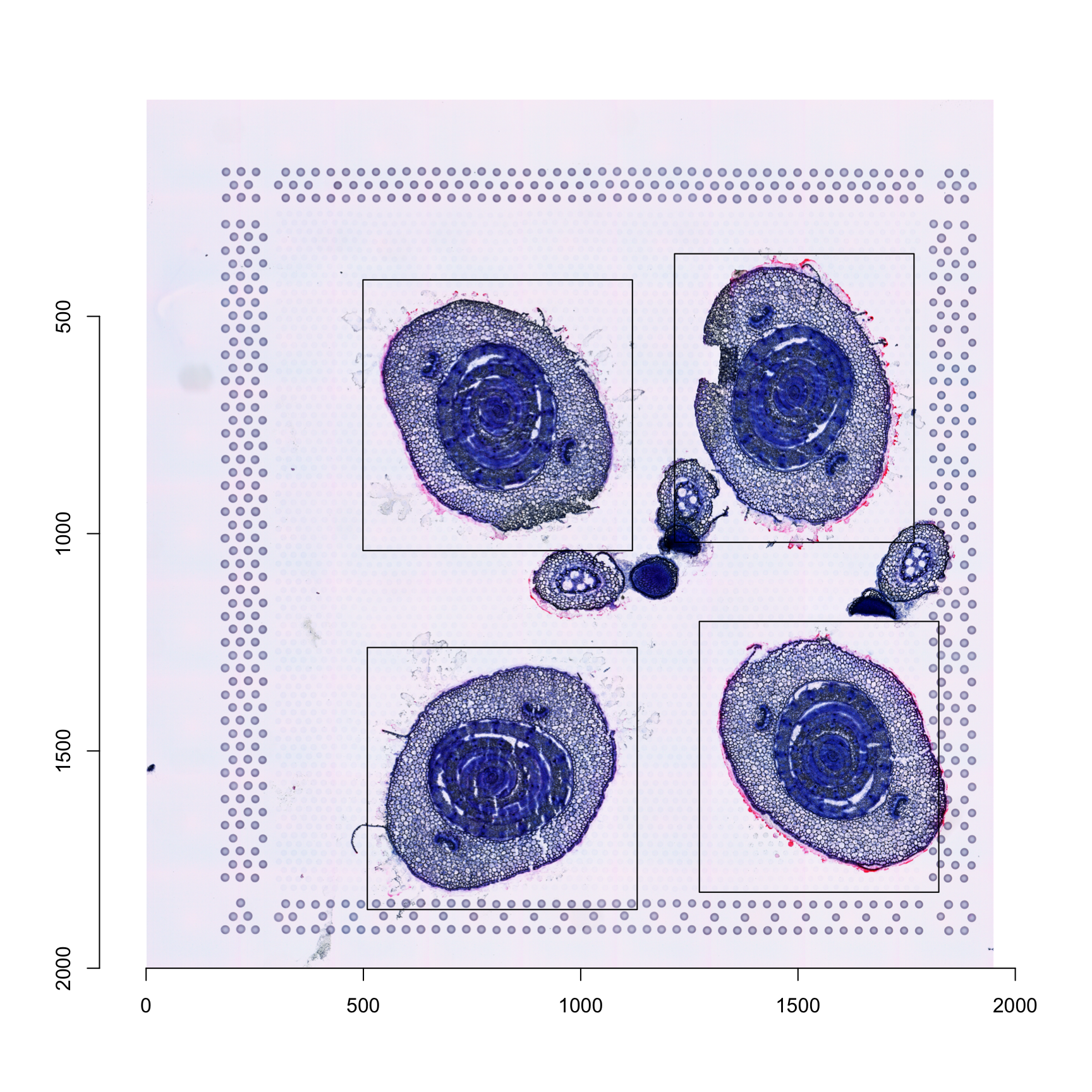
| Version | Author | Date |
|---|---|---|
| 1d8db06 | Ludvig Larsson | 2022-02-28 |
se.cropped <- CropImages(se, crop.geometry.list = crop.geoms, xdim = 500, time.resolve = FALSE, verbose = TRUE)Mask images
Next, we’ll mask the images. The MaskImages default masking function usually works well for HE staining, but in this case we need to resort to a different strategy. Below is an example of a custom masking function that we can use on our tissue images.
se.masked <- readRDS("~/chi_chih/R_objects/se.masked")msk.fkn <- function(im) {
suppressWarnings({
im <- imager::grayscale(im)
im <- imager::isoblur(im, 3)
out <- imager::threshold(im)
out <- !out
out <- imager::fill(out, 5)
out <- EBImage::as.Image(out)
out <- EBImage::fillHull(out)
out <- imager::as.pixset(out)
})
return(out)
}
se.masked <- MaskImages(se.cropped, custom.msk.fkn = msk.fkn, verbose = TRUE)Align images
Next we can align the four tissue sections using the ManualAlignImages function. There are some distortions in the sections which makes it virtually impossible to achieve a good alignment using only rigid transformations. To achieve a decent alignment, we also need to strecth/compress the tissue.
se.masked <- ManualAlignImages(se.masked, fix.axes = TRUE)Here are approximate settings that were used fo the manual alignment.
settings <- data.frame(sample = c(2, 3, 4),
                       rotation_angle = c(-27.7, 88.8, 4.2),
                       shift_x = c(-9, 26, 40),
                       shift_y = c(69, -7, -26),
                       angle_blue = c(27, 0, 37.4),
                       stretch_blue = c(0.92, 1, 0.93),
                       angle_red = c(33.3, 0, 37.4),
                       stretch_red = c(0.87, 1, 0.87),
                       mirror_x = c(FALSE, FALSE, TRUE),
                       mirror_y = c(FALSE, FALSE, TRUE))

DT::datatable(settings)
Below is the result after tissue alignment
ImagePlot(se.masked, ncols = 4, method = "raster")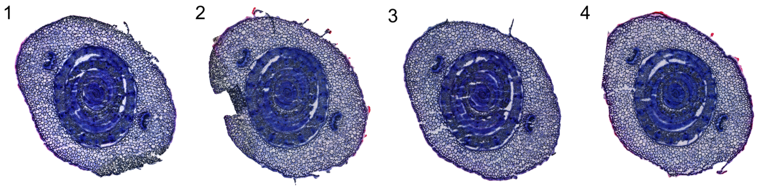
| Version | Author | Date |
|---|---|---|
| 1d8db06 | Ludvig Larsson | 2022-02-28 |
QC
There are slightly higher counts in group1 and group2 which might represent a batch effect, but overall the quality metrics are high.
VlnPlot(se.masked, features = c("nFeature_RNA", "nCount_RNA"), group.by = "labels")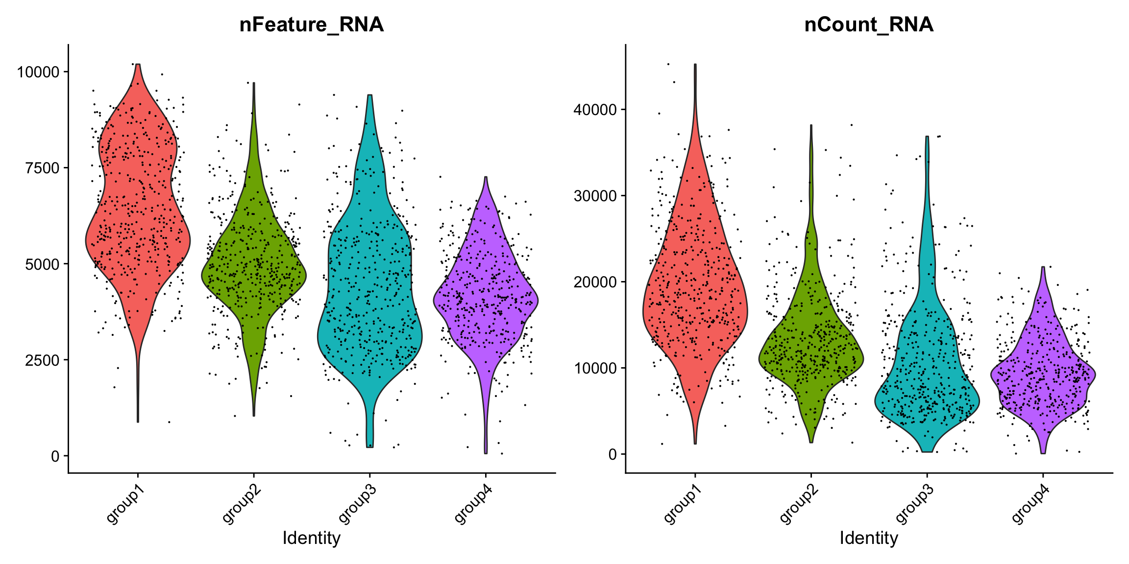
| Version | Author | Date |
|---|---|---|
| 1d8db06 | Ludvig Larsson | 2022-02-28 |
Analysis workflow
Below is a simple analysis workflow based on Seurat functions. For dimensionality reduction we run PCA.
- Normalization with SCTransform
- Dimensionality reduction (PCA)
- UMAP embedding
- Clustering
se.masked <- se.masked %>%
  SCTransform() %>%
  RunPCA() %>%
  RunUMAP(reduction = "pca", dims = 1:30)
se.masked <- se.masked %>%
FindNeighbors(reduction = "pca", dims = 1:30) %>%
FindClusters() %>%
RunUMAP(reduction = "pca", dims = 1:30)
se.masked$seurat_clusters_pca <- se.masked$seurat_clustersClustering
From the UMAP we can see that the sections are not well mixed, indicating that there is a batch effect present in the data. This could of course be biological, but we could try to use an integration technique to find shared structures across the sections.
p1 <- DimPlot(se.masked, group.by = "labels", reduction = "umap")
p2 <- DimPlot(se.masked, group.by = "seurat_clusters_pca", label = TRUE, label.size = 8, reduction = "umap")
p1 - p2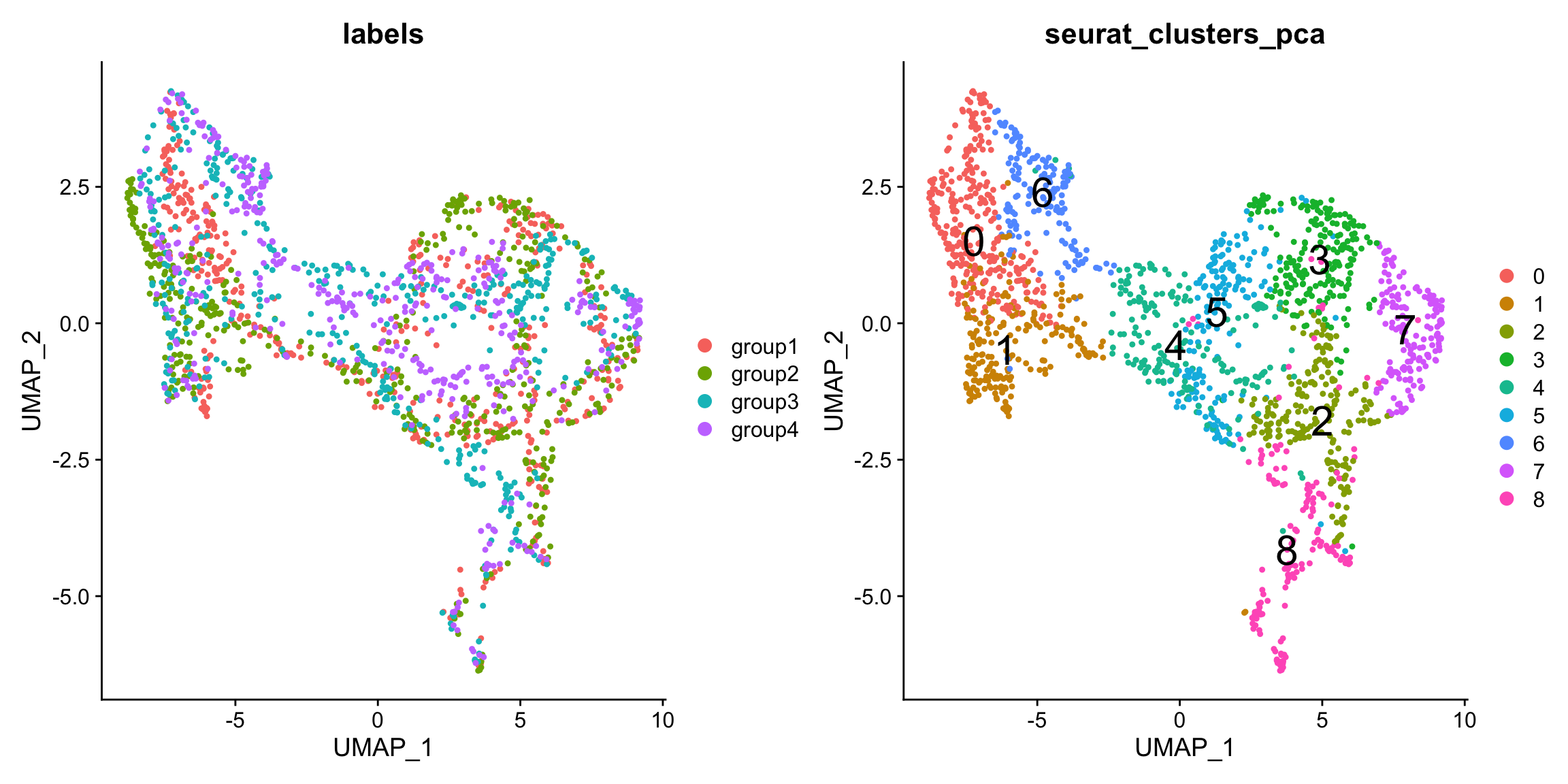
| Version | Author | Date |
|---|---|---|
| 1d8db06 | Ludvig Larsson | 2022-02-28 |
There are also some discrepancies in the spatial distribution of clusters in the different sections.
p1 <- ST.FeaturePlot(se.masked, features = "seurat_clusters_pca", indices = 1, split.labels = T, pt.size = 2) & theme(plot.title = element_blank(), strip.text = element_blank())
p2 <- ST.FeaturePlot(se.masked, features = "seurat_clusters_pca", indices = 2, split.labels = T, pt.size = 2) & theme(plot.title = element_blank(), strip.text = element_blank())
p3 <- ST.FeaturePlot(se.masked, features = "seurat_clusters_pca", indices = 3, split.labels = T, pt.size = 2) & theme(plot.title = element_blank(), strip.text = element_blank())
p4 <- ST.FeaturePlot(se.masked, features = "seurat_clusters_pca", indices = 4, split.labels = T, pt.size = 2) & theme(plot.title = element_blank(), strip.text = element_blank())
cowplot::plot_grid(p1, p2, p3, p4, ncol = 4)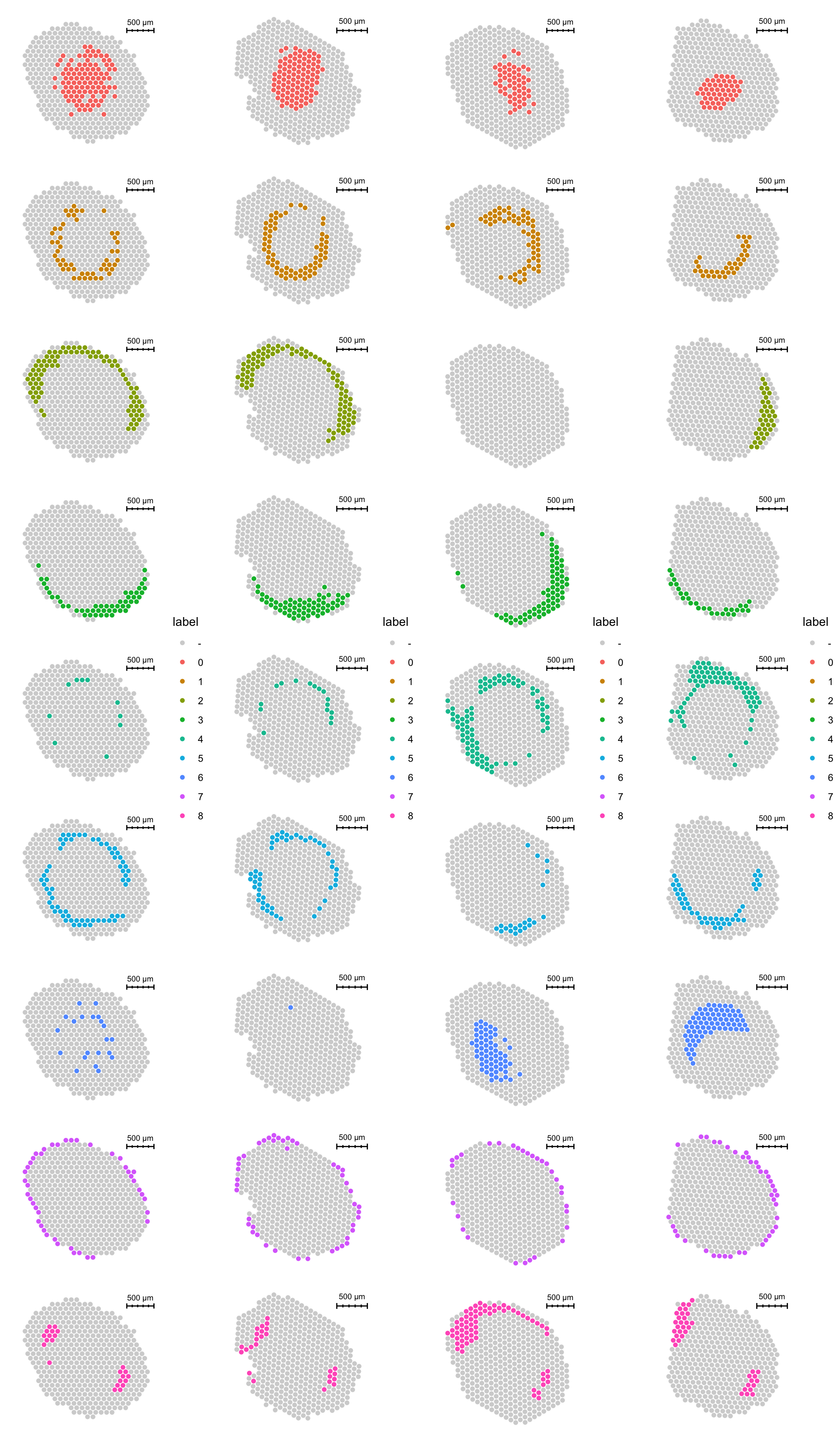
| Version | Author | Date |
|---|---|---|
| 1d8db06 | Ludvig Larsson | 2022-02-28 |
Integrate with harmony
Next, we’ll use harmony to integrate the data from the four sections:
se.masked <- RunHarmony(se.masked, group.by.vars = "labels", reduction = "pca", dims.use = 1:30, assay.use = "SCT", verbose = FALSE) %>%
  RunUMAP(reduction = "harmony", dims = 1:30, reduction.name = "umap.harmony") %>%
  FindNeighbors(reduction = "harmony", dims = 1:30) %>%
  FindClusters()
se.masked$seurat_clusters_harmony <- se.masked$seurat_clusters
After integration, we can see that the four sections are more evenly mixed.
p1 <- DimPlot(se.masked, group.by = "labels", reduction = "umap.harmony")
p2 <- DimPlot(se.masked, group.by = "seurat_clusters_harmony", label = TRUE, label.size = 8, reduction = "umap.harmony")
p1 - p2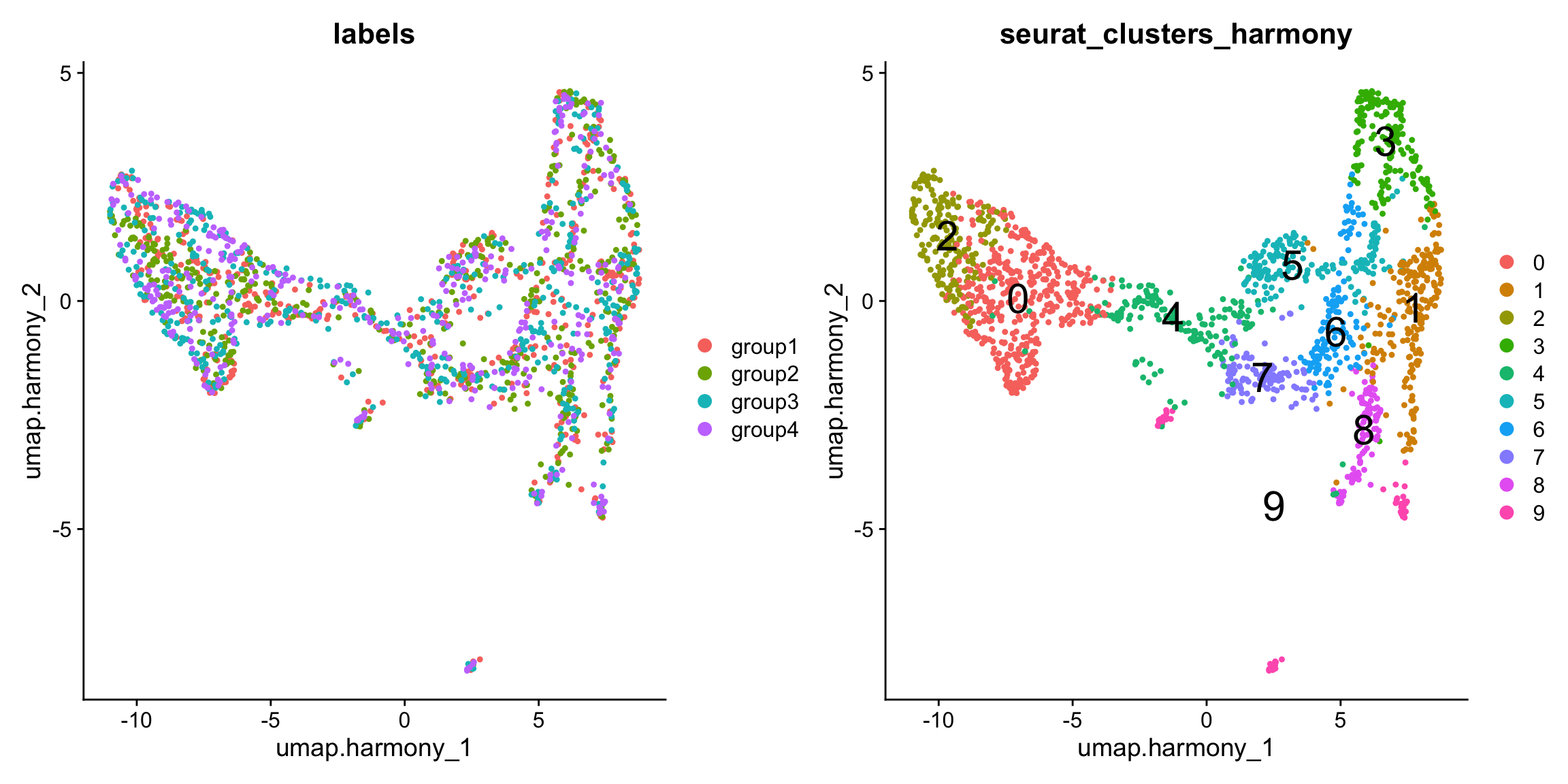
| Version | Author | Date |
|---|---|---|
| 1d8db06 | Ludvig Larsson | 2022-02-28 |
By plotting the clusters on tissue coordinates we can also see that each cluster appearin every tissue section.
p1 <- ST.FeaturePlot(se.masked, features = "seurat_clusters_harmony", indices = 1, split.labels = T, pt.size = 2) & theme(plot.title = element_blank(), strip.text = element_blank())
p2 <- ST.FeaturePlot(se.masked, features = "seurat_clusters_harmony", indices = 2, split.labels = T, pt.size = 2) & theme(plot.title = element_blank(), strip.text = element_blank())
p3 <- ST.FeaturePlot(se.masked, features = "seurat_clusters_harmony", indices = 3, split.labels = T, pt.size = 2) & theme(plot.title = element_blank(), strip.text = element_blank())
p4 <- ST.FeaturePlot(se.masked, features = "seurat_clusters_harmony", indices = 4, split.labels = T, pt.size = 2) & theme(plot.title = element_blank(), strip.text = element_blank())
cowplot::plot_grid(p1, p2, p3, p4, ncol = 4)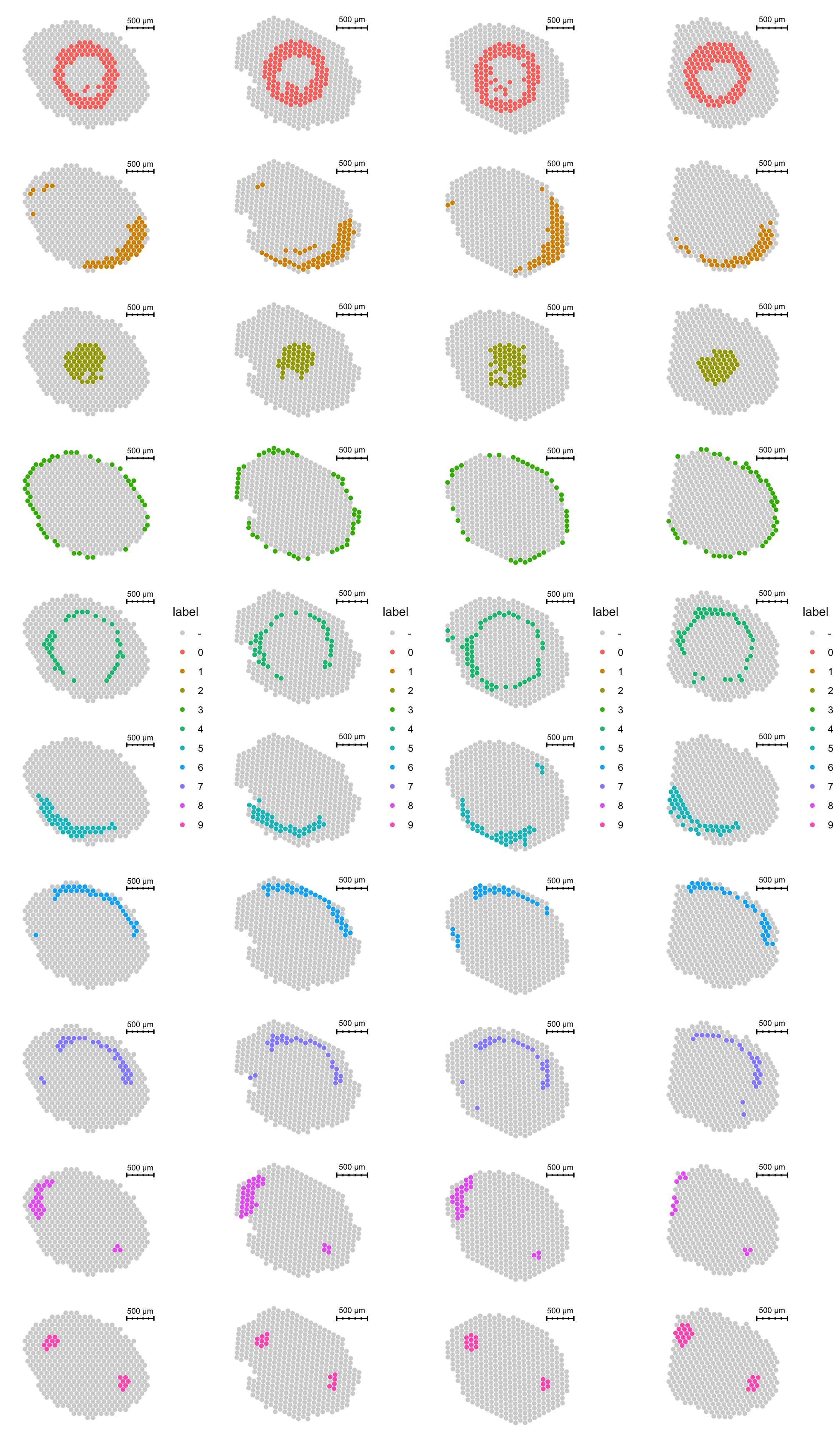
| Version | Author | Date |
|---|---|---|
| 1d8db06 | Ludvig Larsson | 2022-02-28 |
DE analysis
From these clsuetrs, we can extract marker genes by differential expression analysis (DEA).
de.markers <- FindAllMarkers(se.masked, only.pos = TRUE)top10 <- de.markers %>%
dplyr::filter(p_val_adj < 0.01) %>%
dplyr::group_by(cluster) %>%
dplyr::top_n(wt = -p_val_adj, n = 10)
DoHeatmap(se.masked, features = top10$gene)Warning in DoHeatmap(se.masked, features = top10$gene): The following features
were omitted as they were not found in the scale.data slot for the SCT assay:
Zm00001d044529, G2-like-transcription factor 26, cyclin11, ribosomal protein
S27, Zm00001d038374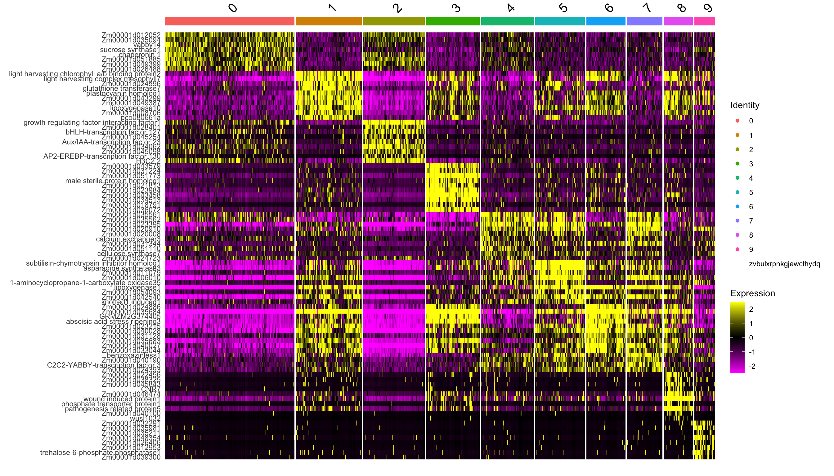
| Version | Author | Date |
|---|---|---|
| 1d8db06 | Ludvig Larsson | 2022-02-28 |
3D stack
By runnig Create3DStack, we can create a z-stack of “2D point patterns” which we’ll use to interpolate expression values over and visualzie expression in 2D space.
se.masked <- Create3DStack(object = se.masked, limit = 0.5, maxnum = 5e3, nx = 200)3D visualization
Now that we have some marker genes we can try to visualize them in 3D
FeaturePlot3D(se.masked, features = "Zm00001d053156")If you don’t want to use the “cell scatter cloud”, you can also just visualize expression at the spot level.
FeaturePlot3D(se.masked, features = "Zm00001d053156", mode = "spots", pt.size = 4, pt.alpha = 0.7)Or do some other fancy tricks to color the sections according to similarities in gene expression for example
se.masked <- RunUMAP(se.masked, dims = 1:30, reduction = "harmony", n.components = 3, reduction.name = "umap.3d")Warning: The default method for RunUMAP has changed from calling Python UMAP via reticulate to the R-native UWOT using the cosine metric
To use Python UMAP via reticulate, set umap.method to 'umap-learn' and metric to 'correlation'
This message will be shown once per session16:44:24 UMAP embedding parameters a = 0.9922 b = 1.11216:44:24 Read 1761 rows and found 30 numeric columns16:44:24 Using Annoy for neighbor search, n_neighbors = 3016:44:24 Building Annoy index with metric = cosine, n_trees = 500% 10 20 30 40 50 60 70 80 90 100%[----|----|----|----|----|----|----|----|----|----|**************************************************|
16:44:24 Writing NN index file to temp file /var/folders/zb/1fj07x_5343fvs_k28gnm1z80002xs/T//Rtmpnu2L29/file4299db0b103
16:44:24 Searching Annoy index using 1 thread, search_k = 3000
16:44:24 Annoy recall = 100%
16:44:25 Commencing smooth kNN distance calibration using 1 thread
16:44:27 Initializing from normalized Laplacian + noise
16:44:27 Commencing optimization for 500 epochs, with 69192 positive edges
16:44:30 Optimization finishedDimPlot3D(se.masked, dims = 1:3, blend = TRUE, reduction = "umap.3d", mode = "spots", pt.size = 5, pt.alpha = 1)This can of course also be done in 2D
ImagePlot(se.masked, ncols = 4, method = "raster")
| Version | Author | Date |
|---|---|---|
| 1d8db06 | Ludvig Larsson | 2022-02-28 |
ST.DimPlot(se.masked, dims = 1:3, reduction = "umap.3d", blend = TRUE, ncol = 4, pt.size = 3)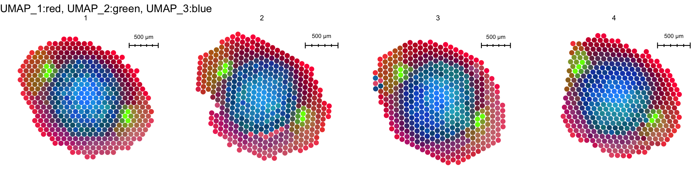
| Version | Author | Date |
|---|---|---|
| 1d8db06 | Ludvig Larsson | 2022-02-28 |
Date
date()[1] "Mon Feb 28 16:44:37 2022"Session Info
devtools::session_info()─ Session info ───────────────────────────────────────────────────────────────
setting value
version R version 4.0.3 (2020-10-10)
os macOS Mojave 10.14.6
system x86_64, darwin13.4.0
ui unknown
language (EN)
collate en_US.UTF-8
ctype en_US.UTF-8
tz Europe/Stockholm
date 2022-02-28
─ Packages ───────────────────────────────────────────────────────────────────
package * version date lib
abind 1.4-5 2016-07-21 [1]
akima 0.6-2.1 2020-05-30 [1]
assertthat 0.2.1 2019-03-21 [1]
BiocGenerics 0.36.0 2020-10-27 [1]
bitops 1.0-7 2021-04-24 [1]
bmp 0.3 2017-09-11 [1]
boot 1.3-27 2021-02-12 [1]
bslib 0.2.4 2021-01-25 [1]
cachem 1.0.4 2021-02-13 [1]
callr 3.7.0 2021-04-20 [1]
class 7.3-18 2021-01-24 [1]
classInt 0.4-3 2020-04-07 [1]
cli 3.1.1 2022-01-20 [1]
cluster 2.1.1 2021-02-14 [1]
coda 0.19-4 2020-09-30 [1]
codetools 0.2-18 2020-11-04 [1]
colorRamps 2.3 2012-10-29 [1]
colorspace 2.0-0 2020-11-11 [1]
cowplot 1.1.1 2020-12-30 [1]
crayon 1.4.1 2021-02-08 [1]
crosstalk 1.1.1 2021-01-12 [1]
data.table 1.14.0 2021-02-21 [1]
DBI 1.1.1 2021-01-15 [1]
dbscan 1.1-6 2021-02-26 [1]
deldir 1.0-6 2021-10-23 [1]
desc 1.3.0 2021-03-05 [1]
devtools 2.4.0 2021-04-07 [1]
digest 0.6.27 2020-10-24 [1]
doParallel 1.0.16 2020-10-16 [1]
dplyr * 1.0.8 2022-02-08 [1]
DT 0.17 2021-01-06 [1]
e1071 1.7-6 2021-03-18 [1]
EBImage * 4.32.0 2020-10-27 [1]
ellipsis 0.3.2 2021-04-29 [1]
evaluate 0.14 2019-05-28 [1]
expm 0.999-6 2021-01-13 [1]
fansi 0.4.2 2021-01-15 [1]
farver 2.1.0 2021-02-28 [1]
fastmap 1.1.0 2021-01-25 [1]
fftwtools 0.9-11 2021-03-01 [1]
fitdistrplus 1.1-3 2020-12-05 [1]
foreach 1.5.1 2020-10-15 [1]
fs 1.5.0 2020-07-31 [1]
future 1.21.0 2020-12-10 [1]
future.apply 1.7.0 2021-01-04 [1]
gdata 2.18.0 2017-06-06 [1]
gdtools 0.2.3 2021-01-06 [1]
generics 0.1.0 2020-10-31 [1]
getPass 0.2-2 2017-07-21 [1]
ggiraph 0.7.8 2020-07-01 [1]
ggplot2 * 3.3.5 2021-06-25 [1]
ggrepel 0.9.1 2021-01-15 [1]
ggridges 0.5.3 2021-01-08 [1]
git2r 0.28.0 2021-01-10 [1]
globals 0.14.0 2020-11-22 [1]
glue 1.4.2 2020-08-27 [1]
gmodels 2.18.1 2018-06-25 [1]
goftest 1.2-2 2019-12-02 [1]
gridExtra 2.3 2017-09-09 [1]
gtable 0.3.0 2019-03-25 [1]
gtools 3.8.2 2020-03-31 [1]
harmony * 1.0 2021-05-11 [1]
highr 0.8 2019-03-20 [1]
htmltools 0.5.1.1 2021-01-22 [1]
htmlwidgets 1.5.3 2020-12-10 [1]
httpuv 1.5.5 2021-01-13 [1]
httr 1.4.2 2020-07-20 [1]
ica 1.0-2 2018-05-24 [1]
igraph 1.2.6 2020-10-06 [1]
imager * 0.42.8 2021-03-15 [1]
irlba 2.3.3 2019-02-05 [1]
iterators 1.0.13 2020-10-15 [1]
jpeg 0.1-8.1 2019-10-24 [1]
jquerylib 0.1.3 2020-12-17 [1]
jsonlite 1.7.2 2020-12-09 [1]
KernSmooth 2.23-18 2020-10-29 [1]
knitr 1.31 2021-01-27 [1]
labeling 0.4.2 2020-10-20 [1]
later 1.1.0.1 2020-06-05 [1]
lattice 0.20-41 2020-04-02 [1]
lazyeval 0.2.2 2019-03-15 [1]
LearnBayes 2.15.1 2018-03-18 [1]
leiden 0.3.7 2021-01-26 [1]
lifecycle 1.0.1 2021-09-24 [1]
listenv 0.8.0 2019-12-05 [1]
lmtest 0.9-38 2020-09-09 [1]
locfit 1.5-9.4 2020-03-25 [1]
magick 2.7.2 2021-05-02 [1]
magrittr * 2.0.1 2020-11-17 [1]
manipulateWidget 0.11.0 2021-05-31 [1]
MASS 7.3-53.1 2021-02-12 [1]
Matrix 1.3-2 2021-01-06 [1]
matrixStats 0.58.0 2021-01-29 [1]
memoise 2.0.0 2021-01-26 [1]
mgcv 1.8-34 2021-02-16 [1]
mime 0.10 2021-02-13 [1]
miniUI 0.1.1.1 2018-05-18 [1]
Morpho 2.8 2020-03-09 [1]
munsell 0.5.0 2018-06-12 [1]
nlme 3.1-152 2021-02-04 [1]
parallelly 1.25.0 2021-04-30 [1]
patchwork 1.1.1 2020-12-17 [1]
pbapply 1.4-3 2020-08-18 [1]
pillar 1.7.0 2022-02-01 [1]
pkgbuild 1.2.0 2020-12-15 [1]
pkgconfig 2.0.3 2019-09-22 [1]
pkgload 1.2.1 2021-04-06 [1]
plotly 4.9.3 2021-01-10 [1]
plyr 1.8.6 2020-03-03 [1]
png 0.1-7 2013-12-03 [1]
polyclip 1.10-0 2019-03-14 [1]
prettyunits 1.1.1 2020-01-24 [1]
processx 3.5.1 2021-04-04 [1]
promises 1.2.0.1 2021-02-11 [1]
proxy 0.4-25 2021-03-05 [1]
ps 1.6.0 2021-02-28 [1]
purrr 0.3.4 2020-04-17 [1]
R6 2.5.0 2020-10-28 [1]
RANN 2.6.1 2019-01-08 [1]
raster 3.4-10 2021-05-03 [1]
RColorBrewer 1.1-2 2014-12-07 [1]
Rcpp * 1.0.6 2021-01-15 [1]
RcppAnnoy 0.0.18 2020-12-15 [1]
RCurl 1.98-1.3 2021-03-16 [1]
readbitmap 0.1.5 2018-06-27 [1]
remotes 2.3.0 2021-04-01 [1]
reshape2 1.4.4 2020-04-09 [1]
reticulate 1.18 2020-10-25 [1]
rgl 0.105.22 2021-03-04 [1]
rlang 1.0.1 2022-02-03 [1]
rmarkdown 2.7 2021-02-19 [1]
ROCR 1.0-11 2020-05-02 [1]
rpart 4.1-15 2019-04-12 [1]
rprojroot 2.0.2 2020-11-15 [1]
RSpectra 0.16-0 2019-12-01 [1]
rstudioapi 0.13 2020-11-12 [1]
Rtsne 0.15 2018-11-10 [1]
Rvcg 0.19.2 2021-01-11 [1]
sass 0.3.1 2021-01-24 [1]
scales 1.1.1 2020-05-11 [1]
scattermore 0.7 2020-11-24 [1]
sctransform 0.3.2 2020-12-16 [1]
sessioninfo 1.1.1 2018-11-05 [1]
Seurat * 4.0.2 2021-06-21 [1]
SeuratObject * 4.0.0 2021-01-15 [1]
sf 0.9-8 2021-03-17 [1]
shiny 1.6.0 2021-01-25 [1]
shinyjs 2.0.0 2020-09-09 [1]
sp 1.4-5 2021-01-10 [1]
spatstat.core 2.3-0 2021-07-16 [1]
spatstat.data 2.1-0 2021-03-21 [1]
spatstat.geom 2.3-0 2021-10-09 [1]
spatstat.sparse 2.0-0 2021-03-16 [1]
spatstat.utils 2.2-0 2021-06-14 [1]
spData 0.3.8 2020-07-03 [1]
spdep 1.1-7 2021-04-03 [1]
stringi 1.5.3 2020-09-09 [1]
stringr 1.4.0 2019-02-10 [1]
STutility * 0.1.0 2022-02-28 [1]
survival 3.2-10 2021-03-16 [1]
systemfonts 1.0.1 2021-02-09 [1]
tensor 1.5 2012-05-05 [1]
testthat 3.0.2 2021-02-14 [1]
tibble 3.1.6 2021-11-07 [1]
tidyr 1.2.0 2022-02-01 [1]
tidyselect 1.1.1 2021-04-30 [1]
tiff 0.1-8 2021-03-31 [1]
units 0.7-1 2021-03-16 [1]
usethis 2.0.1 2021-02-10 [1]
utf8 1.2.1 2021-03-12 [1]
uuid 0.1-4 2020-02-26 [1]
uwot 0.1.10 2020-12-15 [1]
vctrs 0.3.8 2021-04-29 [1]
viridis 0.6.1 2021-05-11 [1]
viridisLite 0.4.0 2021-04-13 [1]
whisker 0.4 2019-08-28 [1]
withr 2.4.1 2021-01-26 [1]
workflowr * 1.7.0 2021-12-21 [1]
xfun 0.20 2021-01-06 [1]
xtable 1.8-4 2019-04-21 [1]
yaml 2.2.1 2020-02-01 [1]
zeallot 0.1.0 2018-01-28 [1]
zoo 1.8-9 2021-03-09 [1]
source
CRAN (R 4.0.0)
CRAN (R 4.0.3)
CRAN (R 4.0.0)
Bioconductor
CRAN (R 4.0.3)
CRAN (R 4.0.3)
CRAN (R 4.0.3)
CRAN (R 4.0.3)
CRAN (R 4.0.3)
CRAN (R 4.0.3)
CRAN (R 4.0.3)
CRAN (R 4.0.3)
CRAN (R 4.0.3)
CRAN (R 4.0.3)
CRAN (R 4.0.2)
CRAN (R 4.0.3)
CRAN (R 4.0.3)
CRAN (R 4.0.3)
CRAN (R 4.0.3)
CRAN (R 4.0.3)
CRAN (R 4.0.3)
CRAN (R 4.0.3)
CRAN (R 4.0.3)
CRAN (R 4.0.3)
CRAN (R 4.0.3)
CRAN (R 4.0.3)
CRAN (R 4.0.3)
CRAN (R 4.0.3)
CRAN (R 4.0.3)
CRAN (R 4.0.3)
CRAN (R 4.0.3)
CRAN (R 4.0.3)
Bioconductor
CRAN (R 4.0.3)
CRAN (R 4.0.0)
CRAN (R 4.0.3)
CRAN (R 4.0.3)
CRAN (R 4.0.3)
CRAN (R 4.0.3)
CRAN (R 4.0.5)
CRAN (R 4.0.3)
CRAN (R 4.0.3)
CRAN (R 4.0.2)
CRAN (R 4.0.3)
CRAN (R 4.0.3)
CRAN (R 4.0.0)
CRAN (R 4.0.3)
CRAN (R 4.0.3)
CRAN (R 4.0.5)
CRAN (R 4.0.3)
CRAN (R 4.0.3)
CRAN (R 4.0.3)
CRAN (R 4.0.3)
CRAN (R 4.0.3)
CRAN (R 4.0.3)
CRAN (R 4.0.3)
CRAN (R 4.0.0)
CRAN (R 4.0.0)
CRAN (R 4.0.0)
CRAN (R 4.0.0)
CRAN (R 4.0.0)
Github (immunogenomics/harmony@c8f4901)
CRAN (R 4.0.0)
CRAN (R 4.0.3)
CRAN (R 4.0.3)
CRAN (R 4.0.3)
CRAN (R 4.0.2)
CRAN (R 4.0.0)
CRAN (R 4.0.3)
CRAN (R 4.0.3)
CRAN (R 4.0.0)
CRAN (R 4.0.3)
CRAN (R 4.0.3)
CRAN (R 4.0.3)
CRAN (R 4.0.3)
CRAN (R 4.0.3)
CRAN (R 4.0.3)
CRAN (R 4.0.3)
CRAN (R 4.0.0)
CRAN (R 4.0.3)
CRAN (R 4.0.0)
CRAN (R 4.0.0)
CRAN (R 4.0.3)
CRAN (R 4.0.3)
CRAN (R 4.0.0)
CRAN (R 4.0.3)
CRAN (R 4.0.3)
CRAN (R 4.0.3)
CRAN (R 4.0.3)
CRAN (R 4.0.3)
CRAN (R 4.0.3)
CRAN (R 4.0.3)
CRAN (R 4.0.3)
CRAN (R 4.0.3)
CRAN (R 4.0.3)
CRAN (R 4.0.3)
CRAN (R 4.0.0)
CRAN (R 4.0.3)
CRAN (R 4.0.0)
CRAN (R 4.0.3)
CRAN (R 4.0.3)
CRAN (R 4.0.3)
CRAN (R 4.0.2)
CRAN (R 4.0.3)
CRAN (R 4.0.3)
CRAN (R 4.0.0)
CRAN (R 4.0.3)
CRAN (R 4.0.3)
CRAN (R 4.0.0)
CRAN (R 4.0.0)
CRAN (R 4.0.0)
CRAN (R 4.0.0)
CRAN (R 4.0.3)
CRAN (R 4.0.3)
CRAN (R 4.0.3)
CRAN (R 4.0.3)
CRAN (R 4.0.0)
CRAN (R 4.0.3)
CRAN (R 4.0.0)
CRAN (R 4.0.3)
CRAN (R 4.0.3)
CRAN (R 4.0.3)
CRAN (R 4.0.3)
CRAN (R 4.0.3)
CRAN (R 4.0.3)
CRAN (R 4.0.3)
CRAN (R 4.0.0)
CRAN (R 4.0.3)
CRAN (R 4.0.3)
CRAN (R 4.0.3)
CRAN (R 4.0.3)
CRAN (R 4.0.0)
CRAN (R 4.0.3)
CRAN (R 4.0.3)
CRAN (R 4.0.0)
CRAN (R 4.0.3)
CRAN (R 4.0.0)
CRAN (R 4.0.3)
CRAN (R 4.0.3)
CRAN (R 4.0.3)
CRAN (R 4.0.3)
CRAN (R 4.0.3)
CRAN (R 4.0.0)
Github (lldelisle/seurat@af2925c)
CRAN (R 4.0.3)
CRAN (R 4.0.3)
CRAN (R 4.0.3)
CRAN (R 4.0.3)
CRAN (R 4.0.3)
CRAN (R 4.0.3)
CRAN (R 4.0.3)
CRAN (R 4.0.3)
CRAN (R 4.0.3)
CRAN (R 4.0.3)
CRAN (R 4.0.2)
CRAN (R 4.0.3)
CRAN (R 4.0.3)
CRAN (R 4.0.0)
local
CRAN (R 4.0.3)
CRAN (R 4.0.3)
CRAN (R 4.0.0)
CRAN (R 4.0.3)
CRAN (R 4.0.3)
CRAN (R 4.0.3)
CRAN (R 4.0.3)
CRAN (R 4.0.3)
CRAN (R 4.0.3)
CRAN (R 4.0.2)
CRAN (R 4.0.3)
CRAN (R 4.0.0)
CRAN (R 4.0.3)
CRAN (R 4.0.3)
CRAN (R 4.0.3)
CRAN (R 4.0.3)
CRAN (R 4.0.0)
CRAN (R 4.0.3)
CRAN (R 4.0.3)
CRAN (R 4.0.3)
CRAN (R 4.0.0)
CRAN (R 4.0.3)
CRAN (R 4.0.3)
CRAN (R 4.0.3)
[1] /Users/ludviglarsson/anaconda3/envs/R4.0/lib/R/libraryA work by Joseph Bergenstråhle and Ludvig Larsson
sessionInfo()R version 4.0.3 (2020-10-10)
Platform: x86_64-apple-darwin13.4.0 (64-bit)
Running under: macOS Mojave 10.14.6
Matrix products: default
BLAS/LAPACK: /Users/ludviglarsson/anaconda3/envs/R4.0/lib/libopenblasp-r0.3.12.dylib
locale:
[1] en_US.UTF-8/en_US.UTF-8/en_US.UTF-8/C/en_US.UTF-8/en_US.UTF-8
attached base packages:
[1] stats graphics grDevices utils datasets methods base
other attached packages:
[1] harmony_1.0 Rcpp_1.0.6 dplyr_1.0.8 STutility_0.1.0
[5] ggplot2_3.3.5 EBImage_4.32.0 imager_0.42.8 magrittr_2.0.1
[9] SeuratObject_4.0.0 Seurat_4.0.2 workflowr_1.7.0
loaded via a namespace (and not attached):
[1] utf8_1.2.1 reticulate_1.18 tidyselect_1.1.1
[4] htmlwidgets_1.5.3 grid_4.0.3 Rtsne_0.15
[7] devtools_2.4.0 munsell_0.5.0 codetools_0.2-18
[10] ica_1.0-2 units_0.7-1 DT_0.17
[13] future_1.21.0 miniUI_0.1.1.1 withr_2.4.1
[16] colorspace_2.0-0 highr_0.8 knitr_1.31
[19] uuid_0.1-4 rstudioapi_0.13 ROCR_1.0-11
[22] tensor_1.5 listenv_0.8.0 labeling_0.4.2
[25] git2r_0.28.0 polyclip_1.10-0 farver_2.1.0
[28] rprojroot_2.0.2 coda_0.19-4 parallelly_1.25.0
[31] LearnBayes_2.15.1 vctrs_0.3.8 generics_0.1.0
[34] xfun_0.20 R6_2.5.0 doParallel_1.0.16
[37] locfit_1.5-9.4 Morpho_2.8 ggiraph_0.7.8
[40] manipulateWidget_0.11.0 cachem_1.0.4 bitops_1.0-7
[43] spatstat.utils_2.2-0 assertthat_0.2.1 promises_1.2.0.1
[46] scales_1.1.1 gtable_0.3.0 globals_0.14.0
[49] bmp_0.3 processx_3.5.1 goftest_1.2-2
[52] rlang_1.0.1 zeallot_0.1.0 akima_0.6-2.1
[55] systemfonts_1.0.1 splines_4.0.3 lazyeval_0.2.2
[58] spatstat.geom_2.3-0 rgl_0.105.22 yaml_2.2.1
[61] reshape2_1.4.4 abind_1.4-5 crosstalk_1.1.1
[64] httpuv_1.5.5 usethis_2.0.1 tools_4.0.3
[67] spData_0.3.8 ellipsis_0.3.2 spatstat.core_2.3-0
[70] raster_3.4-10 jquerylib_0.1.3 RColorBrewer_1.1-2
[73] proxy_0.4-25 BiocGenerics_0.36.0 sessioninfo_1.1.1
[76] Rvcg_0.19.2 ggridges_0.5.3 plyr_1.8.6
[79] classInt_0.4-3 purrr_0.3.4 RCurl_1.98-1.3
[82] prettyunits_1.1.1 ps_1.6.0 rpart_4.1-15
[85] dbscan_1.1-6 deldir_1.0-6 viridis_0.6.1
[88] pbapply_1.4-3 cowplot_1.1.1 zoo_1.8-9
[91] ggrepel_0.9.1 cluster_2.1.1 colorRamps_2.3
[94] fs_1.5.0 RSpectra_0.16-0 data.table_1.14.0
[97] magick_2.7.2 scattermore_0.7 readbitmap_0.1.5
[100] gmodels_2.18.1 lmtest_0.9-38 RANN_2.6.1
[103] whisker_0.4 fitdistrplus_1.1-3 matrixStats_0.58.0
[106] pkgload_1.2.1 patchwork_1.1.1 shinyjs_2.0.0
[109] mime_0.10 fftwtools_0.9-11 evaluate_0.14
[112] xtable_1.8-4 jpeg_0.1-8.1 gridExtra_2.3
[115] testthat_3.0.2 compiler_4.0.3 tibble_3.1.6
[118] KernSmooth_2.23-18 crayon_1.4.1 htmltools_0.5.1.1
[121] mgcv_1.8-34 later_1.1.0.1 spdep_1.1-7
[124] tiff_0.1-8 tidyr_1.2.0 expm_0.999-6
[127] DBI_1.1.1 MASS_7.3-53.1 sf_0.9-8
[130] boot_1.3-27 Matrix_1.3-2 cli_3.1.1
[133] gdata_2.18.0 parallel_4.0.3 igraph_1.2.6
[136] pkgconfig_2.0.3 getPass_0.2-2 sp_1.4-5
[139] plotly_4.9.3 spatstat.sparse_2.0-0 foreach_1.5.1
[142] bslib_0.2.4 stringr_1.4.0 callr_3.7.0
[145] digest_0.6.27 sctransform_0.3.2 RcppAnnoy_0.0.18
[148] spatstat.data_2.1-0 rmarkdown_2.7 leiden_0.3.7
[151] uwot_0.1.10 gdtools_0.2.3 shiny_1.6.0
[154] gtools_3.8.2 lifecycle_1.0.1 nlme_3.1-152
[157] jsonlite_1.7.2 desc_1.3.0 viridisLite_0.4.0
[160] fansi_0.4.2 pillar_1.7.0 lattice_0.20-41
[163] pkgbuild_1.2.0 fastmap_1.1.0 httr_1.4.2
[166] survival_3.2-10 remotes_2.3.0 glue_1.4.2
[169] png_0.1-7 iterators_1.0.13 class_7.3-18
[172] stringi_1.5.3 sass_0.3.1 memoise_2.0.0
[175] irlba_2.3.3 e1071_1.7-6 future.apply_1.7.0