Plots and themes
Last updated: 2022-02-28
Checks: 7 0
Knit directory: STUtility_web_site/
This reproducible R Markdown analysis was created with workflowr (version 1.7.0). The Checks tab describes the reproducibility checks that were applied when the results were created. The Past versions tab lists the development history.
Great! Since the R Markdown file has been committed to the Git repository, you know the exact version of the code that produced these results.
Great job! The global environment was empty. Objects defined in the global environment can affect the analysis in your R Markdown file in unknown ways. For reproduciblity it’s best to always run the code in an empty environment.
The command set.seed(20191031) was run prior to running the code in the R Markdown file. Setting a seed ensures that any results that rely on randomness, e.g. subsampling or permutations, are reproducible.
Great job! Recording the operating system, R version, and package versions is critical for reproducibility.
Nice! There were no cached chunks for this analysis, so you can be confident that you successfully produced the results during this run.
Great job! Using relative paths to the files within your workflowr project makes it easier to run your code on other machines.
Great! You are using Git for version control. Tracking code development and connecting the code version to the results is critical for reproducibility.
The results in this page were generated with repository version 64ae8be. See the Past versions tab to see a history of the changes made to the R Markdown and HTML files.
Note that you need to be careful to ensure that all relevant files for the analysis have been committed to Git prior to generating the results (you can use wflow_publish or wflow_git_commit). workflowr only checks the R Markdown file, but you know if there are other scripts or data files that it depends on. Below is the status of the Git repository when the results were generated:
Ignored files:
    Ignored:    .Rhistory
    Ignored:    analysis/.DS_Store
    Ignored:    analysis/manual_annotation.png
    Ignored:    pre_data/
Note that any generated files, e.g. HTML, png, CSS, etc., are not included in this status report because it is ok for generated content to have uncommitted changes.
These are the previous versions of the repository in which changes were made to the R Markdown (analysis/Plots_and_Themes.Rmd) and HTML (docs/Plots_and_Themes.html) files. If you’ve configured a remote Git repository (see ?wflow_git_remote), click on the hyperlinks in the table below to view the files as they were in that past version.
| File | Version | Author | Date | Message |
|---|---|---|---|---|
| html | d41bcb0 | Ludvig Larsson | 2022-02-28 | Build site. |
| html | 0dafcee | Ludvig Larsson | 2021-05-06 | Build site. |
| Rmd | b7a0414 | Ludvig Larsson | 2021-05-06 | Updated tutorials |
Patchwork
Many of the plots generated with vsiualization functions from STutility are built using the patchwork R package. This package makes it much easier to change the layout and themes of different plots and we’ll go through a couple of examples here.
Let’s draw a spatial distribution of Pvalb and Th using ST.FeaturePlot and a violin plot showing the expression of these genes within each clusters.
Some of the layout options can be controlled direclty from ST.FeaturePlot using for example ncol and grid.ncol, but you can also rearrange the plot afterwards. Here we set ncol = 2 to specify that the sections will be arranged in two columns and grid.ncol = 1 to specify that the features will be arranged in 1 column.
p1 <- ST.FeaturePlot(se, features = c("Pvalb", "Th"), ncol = 2, grid.ncol = 1)

p1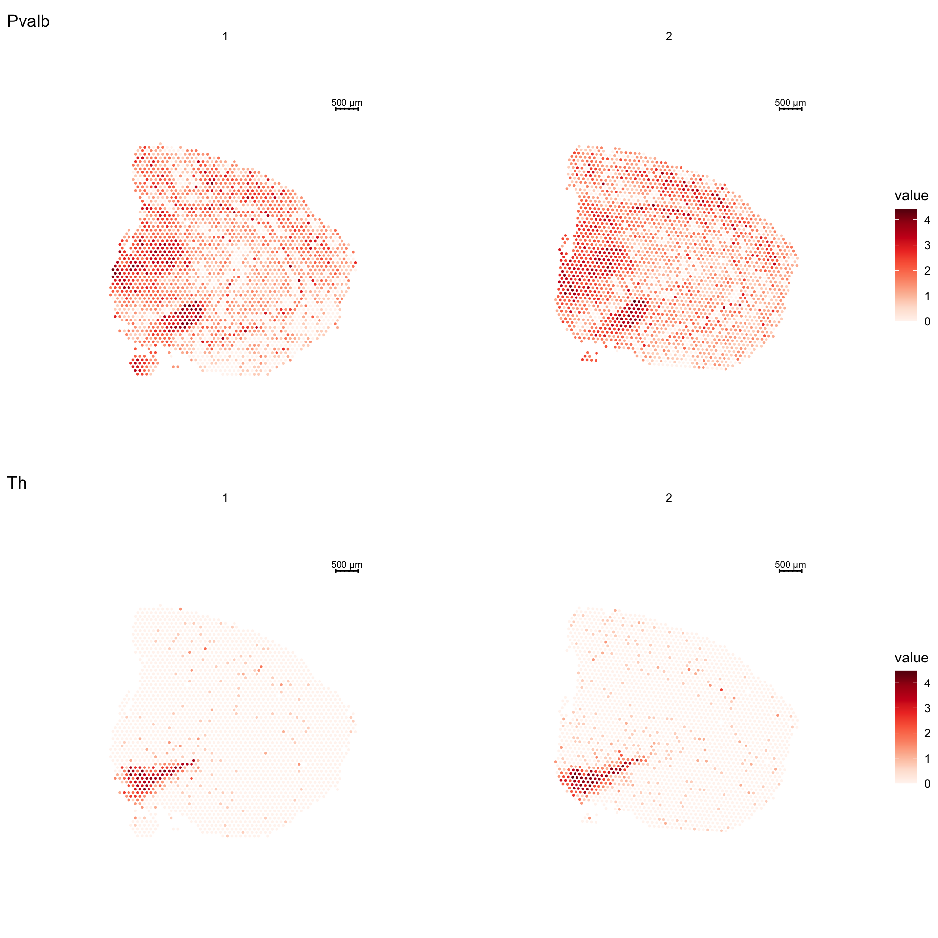
| Version | Author | Date |
|---|---|---|
| 0dafcee | Ludvig Larsson | 2021-05-06 |
Now let’s add a violin plot and show it side by side with the spatial feature plot.
p2 <- VlnPlot(se, features = c("Pvalb", "Th"), ncol = 1, group.by = "seurat_clusters")

p1 - p2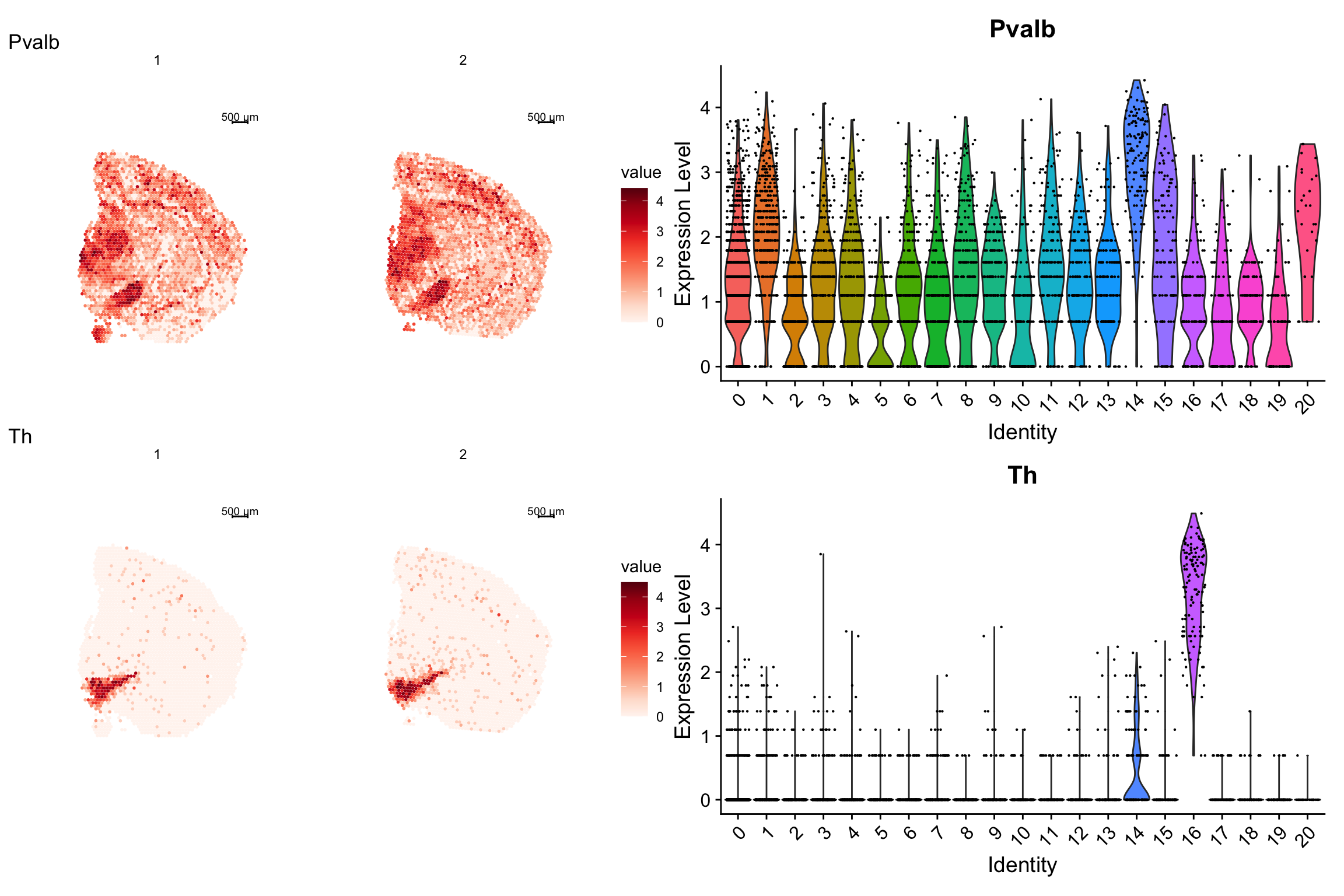
As you can see, it is very easy to combine plots side by side. If you want the sub plots to take up more or less area of the total plot, you can specify layout options with the patchwork function plot_layout.
p1 <- ST.FeaturePlot(se, features = c("Pvalb", "Th"), grid.ncol = 1, indices = 1)
p2 <- VlnPlot(se, features = c("Pvalb", "Th"), ncol = 1, group.by = "seurat_clusters")

# Give the second plot with a width that is 2x the width of the first
p1 - p2 + patchwork::plot_layout(widths = c(1, 2))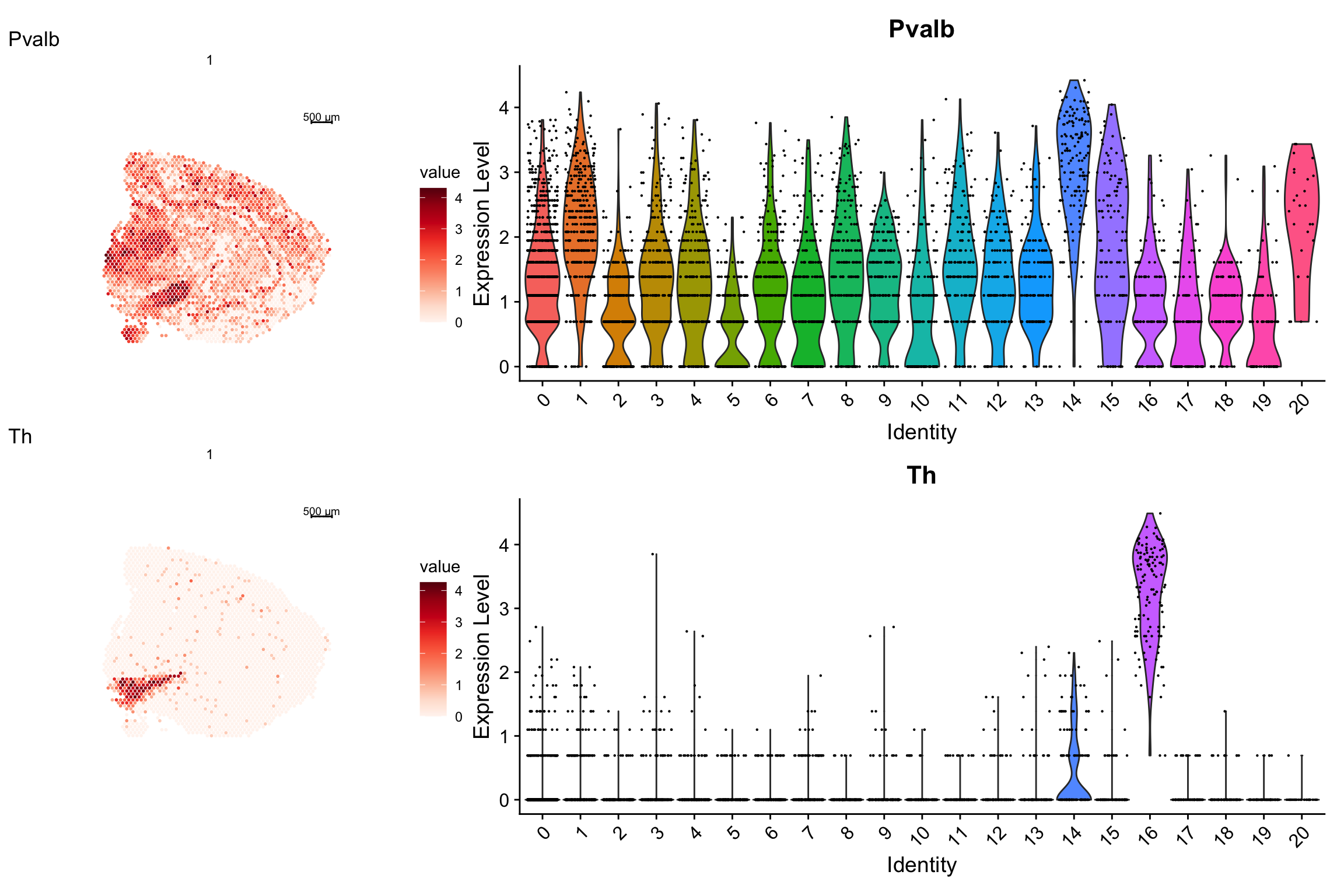
Or an even more complex example
p3 <- ST.FeaturePlot(se, features = c("Pvalb", "Th"), ncol = 2, grid.ncol = 2, show.sb = FALSE)
p1 <- FeaturePlot(se, features = c("Pvalb", "Th"), cols = c("mistyrose", "red", "darkred"))
p2 <- VlnPlot(se, features = c("Pvalb", "Th"), ncol = 2, group.by = "seurat_clusters")

(p1 - p2)/p3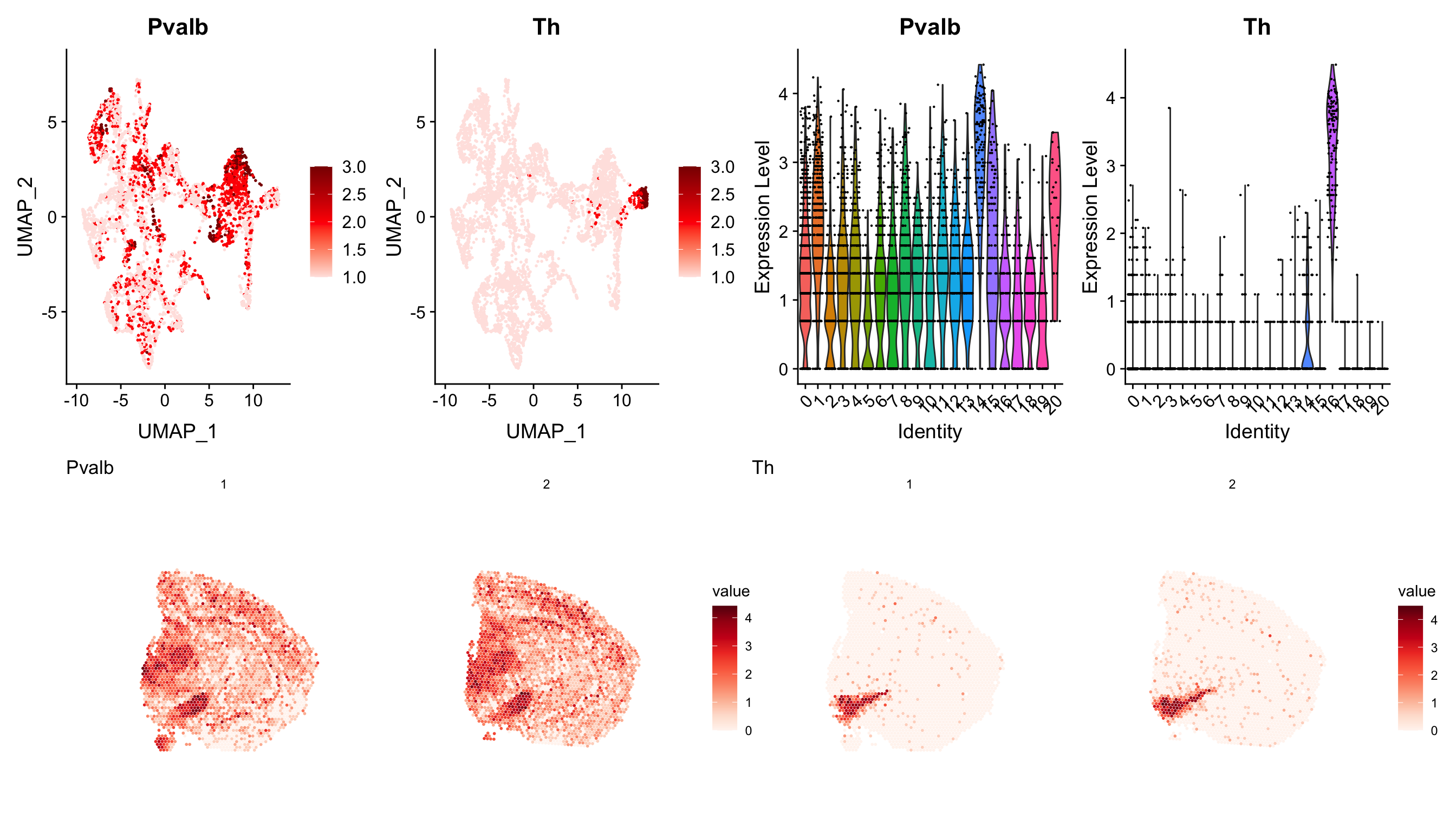
Themes
It is also easy to change the theme of your plots, even after it has been drawn. You can specify a custom theme using the custom.theme argument in ST.FeaturePlot, FeatureOverlay, etc. But it’s even easier with the patchwork system.
custom_theme <- theme(legend.position = c(0.45, 0.8), # Move color legend to top
                      legend.direction = "horizontal", # Flip legend
                      legend.text = element_text(angle = 30, hjust = 1), # rotate legend axis text
                      strip.text = element_blank(), # remove strip text
                      plot.title = element_blank(), # remove plot title
                      plot.margin = margin(t = 0, r = 0, b = 0, l = 0, unit = "cm")) # remove plot margins

p <- ST.FeaturePlot(se, features = "nFeature_RNA", ncol = 2, show.sb = FALSE, palette = "Spectral")
p & custom_theme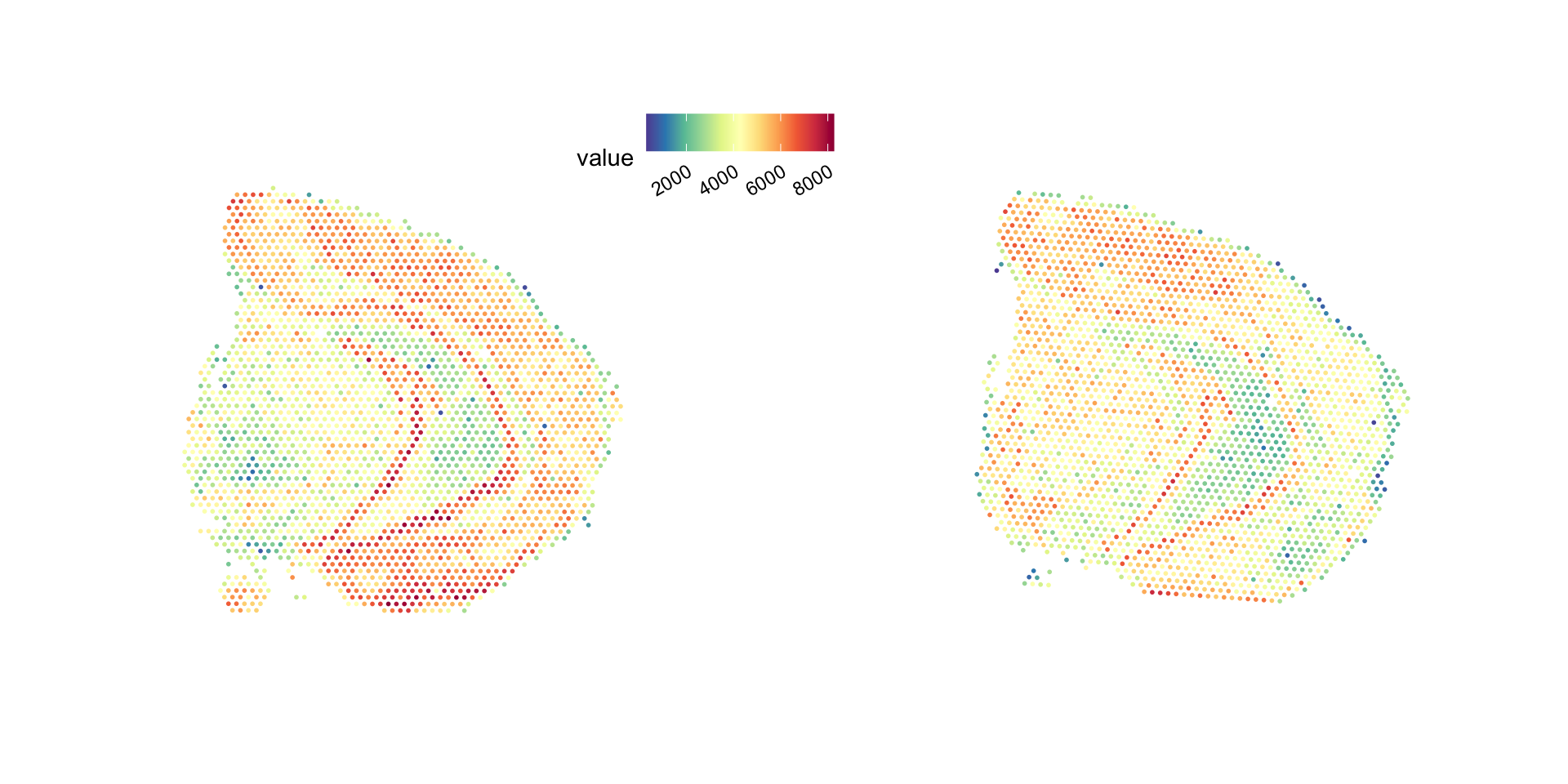
| Version | Author | Date |
|---|---|---|
| 0dafcee | Ludvig Larsson | 2021-05-06 |
Or you can for example add a grid to show the x/y axes. Here, the x/y axes reoresent the pixel coordinates mapped to the “tissue_hires_image.png” from the spaceranger output.
p & theme_bw()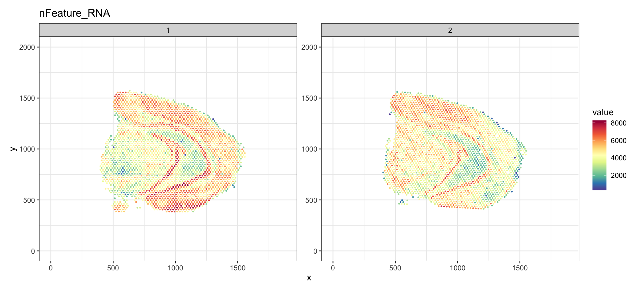
| Version | Author | Date |
|---|---|---|
| 0dafcee | Ludvig Larsson | 2021-05-06 |
A work by Joseph Bergenstråhle and Ludvig Larsson
sessionInfo()R version 4.0.3 (2020-10-10)
Platform: x86_64-apple-darwin13.4.0 (64-bit)
Running under: macOS Mojave 10.14.6
Matrix products: default
BLAS/LAPACK: /Users/ludviglarsson/anaconda3/envs/R4.0/lib/libopenblasp-r0.3.12.dylib
locale:
[1] en_US.UTF-8/en_US.UTF-8/en_US.UTF-8/C/en_US.UTF-8/en_US.UTF-8
attached base packages:
[1] stats graphics grDevices utils datasets methods base
other attached packages:
[1] magrittr_2.0.1 kableExtra_1.3.4 STutility_0.1.0 ggplot2_3.3.5
[5] SeuratObject_4.0.0 Seurat_4.0.2 workflowr_1.7.0
loaded via a namespace (and not attached):
[1] utf8_1.2.1 reticulate_1.18 tidyselect_1.1.1
[4] htmlwidgets_1.5.3 grid_4.0.3 Rtsne_0.15
[7] munsell_0.5.0 codetools_0.2-18 ica_1.0-2
[10] units_0.7-1 future_1.21.0 miniUI_0.1.1.1
[13] withr_2.4.1 colorspace_2.0-0 highr_0.8
[16] knitr_1.31 uuid_0.1-4 rstudioapi_0.13
[19] ROCR_1.0-11 tensor_1.5 listenv_0.8.0
[22] labeling_0.4.2 git2r_0.28.0 polyclip_1.10-0
[25] farver_2.1.0 rprojroot_2.0.2 coda_0.19-4
[28] parallelly_1.25.0 LearnBayes_2.15.1 vctrs_0.3.8
[31] generics_0.1.0 xfun_0.20 R6_2.5.0
[34] doParallel_1.0.16 Morpho_2.8 ggiraph_0.7.8
[37] manipulateWidget_0.11.0 spatstat.utils_2.2-0 assertthat_0.2.1
[40] promises_1.2.0.1 scales_1.1.1 imager_0.42.8
[43] gtable_0.3.0 globals_0.14.0 bmp_0.3
[46] processx_3.5.1 goftest_1.2-2 rlang_1.0.1
[49] zeallot_0.1.0 akima_0.6-2.1 systemfonts_1.0.1
[52] splines_4.0.3 lazyeval_0.2.2 spatstat.geom_2.3-0
[55] rgl_0.105.22 yaml_2.2.1 reshape2_1.4.4
[58] abind_1.4-5 crosstalk_1.1.1 httpuv_1.5.5
[61] tools_4.0.3 spData_0.3.8 ellipsis_0.3.2
[64] spatstat.core_2.3-0 raster_3.4-10 jquerylib_0.1.3
[67] RColorBrewer_1.1-2 proxy_0.4-25 Rvcg_0.19.2
[70] ggridges_0.5.3 Rcpp_1.0.6 plyr_1.8.6
[73] classInt_0.4-3 purrr_0.3.4 ps_1.6.0
[76] rpart_4.1-15 dbscan_1.1-6 deldir_1.0-6
[79] pbapply_1.4-3 viridis_0.6.1 cowplot_1.1.1
[82] zoo_1.8-9 ggrepel_0.9.1 cluster_2.1.1
[85] colorRamps_2.3 fs_1.5.0 data.table_1.14.0
[88] magick_2.7.2 scattermore_0.7 readbitmap_0.1.5
[91] gmodels_2.18.1 lmtest_0.9-38 RANN_2.6.1
[94] whisker_0.4 fitdistrplus_1.1-3 matrixStats_0.58.0
[97] patchwork_1.1.1 shinyjs_2.0.0 mime_0.10
[100] evaluate_0.14 xtable_1.8-4 jpeg_0.1-8.1
[103] gridExtra_2.3 compiler_4.0.3 tibble_3.1.6
[106] KernSmooth_2.23-18 crayon_1.4.1 htmltools_0.5.1.1
[109] mgcv_1.8-34 later_1.1.0.1 spdep_1.1-7
[112] tiff_0.1-8 tidyr_1.2.0 expm_0.999-6
[115] DBI_1.1.1 MASS_7.3-53.1 sf_0.9-8
[118] boot_1.3-27 Matrix_1.3-2 cli_3.1.1
[121] gdata_2.18.0 parallel_4.0.3 igraph_1.2.6
[124] pkgconfig_2.0.3 getPass_0.2-2 sp_1.4-5
[127] plotly_4.9.3 spatstat.sparse_2.0-0 xml2_1.3.2
[130] foreach_1.5.1 svglite_2.0.0 bslib_0.2.4
[133] webshot_0.5.2 rvest_1.0.0 stringr_1.4.0
[136] callr_3.7.0 digest_0.6.27 sctransform_0.3.2
[139] RcppAnnoy_0.0.18 spatstat.data_2.1-0 rmarkdown_2.7
[142] leiden_0.3.7 uwot_0.1.10 gdtools_0.2.3
[145] shiny_1.6.0 gtools_3.8.2 lifecycle_1.0.1
[148] nlme_3.1-152 jsonlite_1.7.2 viridisLite_0.4.0
[151] fansi_0.4.2 pillar_1.7.0 lattice_0.20-41
[154] fastmap_1.1.0 httr_1.4.2 survival_3.2-10
[157] glue_1.4.2 png_0.1-7 iterators_1.0.13
[160] class_7.3-18 stringi_1.5.3 sass_0.3.1
[163] dplyr_1.0.8 irlba_2.3.3 e1071_1.7-6
[166] future.apply_1.7.0